Differentiable Volume Rendering for a Single Ray in Python

Welcome back. In our previous lesson, we constructed the positional encoding function, the crucial first step in the NeRF pipeline that transforms low-dimensional coordinates into a high-dimensional feature space capable of representing fine detail. You now have a function that takes a 5D coordinate $(\mathbf{x},\mathbf{d})$ and prepares it for our neural network.

Today, we will build the final piece of the rendering puzzle: the function that takes the network's output and produces a single pixel color. We'll dive into the physics of how light travels through a participating medium, derive the governing integral equation from first principles, and then implement its discrete, differentiable approximation in Python. This is the heart of NeRF's view synthesis process.

The Physics of Rendering a Semi-Transparent Volume

Before we touch any mathematics, let's build an intuitive physical model. Imagine a camera ray traveling through a cloud of smoke. The final color of the pixel corresponding to this ray is determined by the accumulation of light along its path. As a ray travels, two fundamental phenomena occur:

1. Emission: Particles in the volume (the smoke) might glow, adding light to the ray.
2. Absorption: Particles can also block or absorb light that is traveling from farther away, preventing it from reaching the camera.

The NeRF MLP learns a function that, for any point in space, predicts the properties of the "particle" at that location. Specifically, it outputs:

• Volume Density ($\sigma$): How likely the ray is to interact with a particle at this point. A high $\sigma$ means the point is very opaque, like dense smoke. A low $\sigma$ means it's nearly transparent.
• Color ($\mathbf{c}$): The color of the light that would be emitted from this point in a specific direction.

The following video from Cem Yuksel's graphics course, which you're already familiar with, provides an excellent explanation of these physical interactions that form the basis of the rendering equation.

From Physics to Continuous Integral

Now, let's formalize this intuition. Consider a single camera ray, parameterized as $\mathbf{r}(t)=\mathbf{o}+t\mathbf{d}$, where $\mathbf{o}$ is the camera origin and $\mathbf{d}$ is the ray direction. The ray travels from a near plane $t_n$ to a far plane $t_f$.

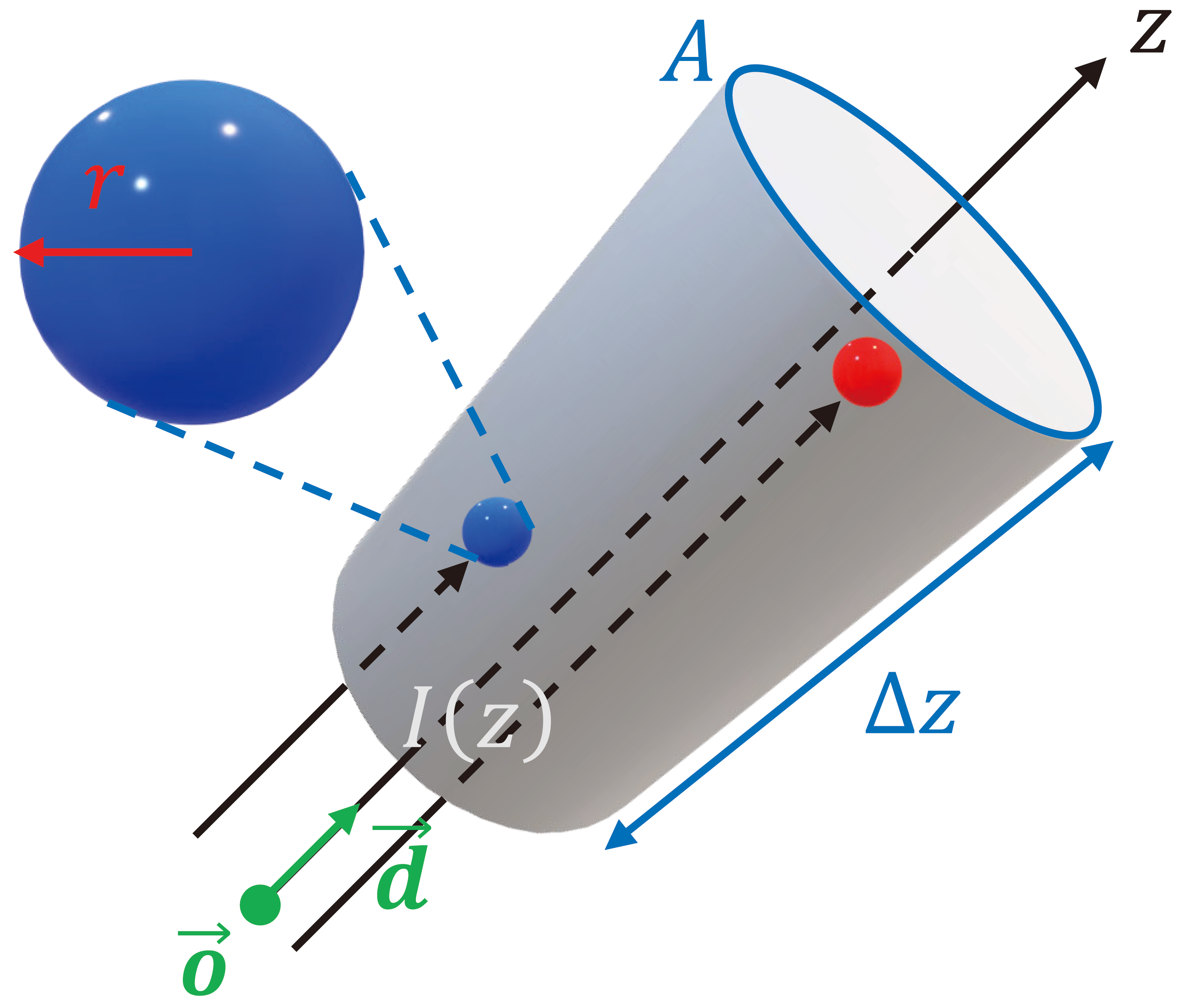
The key quantity we need is transmittance, $T(t)$, which is the probability that a ray travels from $t_n$ to a point $t$ without hitting any particles. It describes how much light from background objects can "shine through" the medium up to point $t$. Transmittance is governed by the volume density $\sigma$. The change in transmittance over an infinitesimally small step $ds$ is proportional to the density at that point: $dT=-T(s)\sigma (s)ds$. Solving this ordinary differential equation gives us the integral form:

The color seen by the camera, $C(\mathbf{r})$, is the integral of all light emitted along the ray, with each point's contribution weighted by its transmittance. The light emitted at point $t$ is given by $\sigma (\mathbf{r}(t))\mathbf{c}(\mathbf{r}(t),\mathbf{d})$. The term $\sigma (\mathbf{r}(t))$ can be interpreted as the differential probability that the ray stops at $t$, releasing color $\mathbf{c}$.

This leads to the volume rendering equation:

For a more rigorous step-by-step derivation of this equation from first principles, the following article is an excellent resource.

From Continuous to Discrete: Numerical Approximation

Computers cannot evaluate continuous integrals. We must approximate them using a numerical method. The NeRF paper uses numerical quadrature. The idea is to split the continuous ray into a finite number of segments and sum up the contributions from each segment.

We take $N$ samples along the ray at depths $\{t_1,t_2,\dots ,t_N\}$. We assume the volume properties ($\sigma$ and $\mathbf{c}$) are constant within each segment $[t_i,t_{i+1}]$.

The integral is now a sum:

Let's dissect this formula, which is the cornerstone of NeRF's rendering:

• ${\delta }_i=t_{i+1}-t_i$ is the distance between adjacent samples.
• ${\sigma }_i$ and ${\mathbf{c}}_i$ are the density and color predicted by the MLP for the $i$-th sample.
• Opacity (${\alpha }_i$): The term ${\alpha }_i=1-\exp (-{\sigma }_i{\delta }_i)$ represents the opacity of the $i$-th segment. It's the probability that light interacts with the volume in this segment. If density ${\sigma }_i$ or length ${\delta }_i$ is high, ${\alpha }_i\to 1$ (opaque). If both are low, ${\alpha }_i\to 0$ (transparent).
• Discrete Transmittance ($T_i$): The term $T_i=\exp \left(-{\sum }_{j=1}^{i-1}{\sigma }_j{\delta }_j\right)$ is the probability that the ray reaches the $i$-th segment without being absorbed. This is the accumulated transparency of all preceding segments.

This formulation is identical to classic alpha compositing used in computer graphics. The final color is a weighted sum of the colors of the samples, where the weight for sample $i$ is $w_i=T_i{\alpha }_i$. This weight represents the probability that the ray travels unimpeded to segment $i$ and then interacts with a particle within that segment.

The following reading walks through this discretization process and explicitly makes the connection to alpha compositing.

Implementing Differentiable Volume Rendering

Now, let's implement this rendering function from scratch. We'll create a Python function that takes the raw outputs from our (hypothetical) MLP for a single ray and computes the final pixel color.

Socratic Question: In the raw2outputs function in the PyTorch code you've seen, dists is calculated as z_vals[..., 1:] - z_vals[..., :-1]. This results in a tensor with one fewer element than the number of samples. The code then concatenates a large value (e.g., 1e10) to the end of the dists tensor. What is the physical interpretation of this large value, and why is it a necessary computational step for this specific formulation?

Here is the complete implementation of the volume rendering function for a batch of rays. We'll follow the structure of the raw2outputs function found in many NeRF implementations.

import torch
import torch.nn.functional as F

def render_rays(raw_outputs, z_vals, ray_directions):
    """
    Transforms raw NeRF output into RGB and other maps.

    Args:
        raw_outputs (torch.Tensor): Raw outputs from the MLP. Shape: (N_rays, N_samples, 4).
                                  The last dimension is [R, G, B, sigma].
        z_vals (torch.Tensor): Integration distances. Shape: (N_rays, N_samples).
        ray_directions (torch.Tensor): Directions of the rays. Shape: (N_rays, 3).

    Returns:
        dict: A dictionary containing:
              'rgb_map': The final rendered RGB color for each ray. Shape: (N_rays, 3).
              'depth_map': The expected depth for each ray. Shape: (N_rays,).
              'acc_map': The accumulated opacity for each ray. Shape: (N_rays,).
              'weights': The weights assigned to each sample. Shape: (N_rays, N_samples).
    """



    # 1. Calculate distances between adjacent samples
    dists = z_vals[..., 1:] - z_vals[..., :-1]
    



    # The distance for the last interval is assumed to be infinite.
    # We append a large value to match the number of samples.
    # This ensures that the accumulated transmittance will eventually go to 0.
    dists = torch.cat([dists, torch.full_like(dists[..., :1], 1e10)], dim=-1) # (N_rays, N_samples)




    # Multiply distance by the norm of the ray direction to get real world distance.
    # This is important if ray_directions are not unit vectors.
    dists = dists * torch.linalg.norm(ray_directions[..., None, :], dim=-1)




    # 2. Extract RGB and sigma from raw MLP output
    # RGB is activated with sigmoid, density with ReLU
    rgb = torch.sigmoid(raw_outputs[..., :3])  # (N_rays, N_samples, 3)
    sigma = F.relu(raw_outputs[..., 3])     # (N_rays, N_samples)




    # 3. Calculate alpha (opacity) for each sample
    # alpha = 1 - exp(-sigma * delta)
    alpha = 1. - torch.exp(-sigma * dists) # (N_rays, N_samples)




    # 4. Calculate weights for each sample
    # T_i = exp(-sum_{j<i} sigma_j * delta_j)
    # The term (1. - alpha) is the transmittance of a single segment.
    # torch.cumprod computes the cumulative product of these transmittances.
    



    # We add a small epsilon (1e-10) for numerical stability.
    # T_i = cumprod(1 - alpha_j + eps) for j < i
    transmittance = torch.cumprod(torch.cat([
        torch.ones_like(alpha[..., :1]), # Transmittance at the start is 1
        1. - alpha + 1e-10
    ], dim=-1), dim=-1)[..., :-1]




    # weight_i = T_i * alpha_i
    weights = alpha * transmittance # (N_rays, N_samples)




    # 5. Compute the final RGB color for the ray
    # C(r) = sum(w_i * c_i)
    rgb_map = torch.sum(weights[..., None] * rgb, dim=-2)  # (N_rays, 3)




    # 6. Compute other useful maps
    # Expected depth is the weighted sum of sample depths.
    depth_map = torch.sum(weights * z_vals, dim=-1)




    # Accumulated opacity is the sum of all weights.
    # This represents the probability that the ray hit something.
    acc_map = torch.sum(weights, -1)
    



    # You can add a white background if the object is on a white canvas
    # rgb_map = rgb_map + (1. - acc_map[..., None])

    return {
        'rgb_map': rgb_map,
        'depth_map': depth_map,
        'acc_map': acc_map,
        'weights': weights
    }




# --- DEMONSTRATION ---




# Define some parameters for a batch of 2 rays
N_rays = 2
N_samples = 64




# Generate dummy MLP outputs (as if they came from the network)
# Shape: (N_rays, N_samples, 4) -> [R, G, B, sigma]
raw_outputs = torch.randn(N_rays, N_samples, 4)




# Generate dummy z_vals (depths) for the samples along the rays
# Linearly spaced between near (2.0) and far (6.0) planes
z_vals = torch.linspace(2.0, 6.0, N_samples).expand(N_rays, N_samples)




# Generate dummy ray directions
ray_directions = torch.randn(N_rays, 3)
ray_directions = ray_directions / torch.linalg.norm(ray_directions, dim=-1, keepdim=True)




# Run the rendering function
rendered_maps = render_rays(raw_outputs, z_vals, ray_directions)




# Print the shapes of the results
print("--- Volume Rendering Output Shapes ---")
for key, value in rendered_maps.items():
    print(f"{key:>10s}: {value.shape}")
print("-" * 36)




# Example output for the first ray
print("\n--- Example Output for First Ray ---")
print(f"Final RGB color: {rendered_maps['rgb_map'][0].tolist()}")
print(f"Expected depth:  {rendered_maps['depth_map'][0].item()}")
print("-" * 36)

This code directly translates the discrete volume rendering equation into a series of vectorized PyTorch operations. Every operation used—multiplication, exponentiation, summation, cumulative product—is differentiable, which is precisely why we can train the NeRF MLP end-to-end by backpropagating the error from the final pixel color all the way back to the network's weights.

Conclusion

In this lesson, you have bridged the gap between the physics of light transport and a practical, differentiable rendering algorithm. This function is the engine that allows NeRF to synthesize images from a neural representation.

Key Takeaways:

• The continuous volume rendering equation mathematically describes how light is accumulated along a ray traveling through a semi-transparent medium.
• This integral is approximated with a discrete sum (numerical quadrature), which is computationally tractable.
• The discrete formula is equivalent to alpha compositing, a standard computer graphics technique, where the final color is a weighted sum of sample colors: $\hat{C}(\mathbf{r})=\sum w_i{\mathbf{c}}_i$.
• The weights, $w_i=T_i{\alpha }_i$, are products of the sample's opacity (${\alpha }_i$) and the accumulated transmittance up to that sample ($T_i$).
• The entire rendering process can be implemented using a chain of differentiable PyTorch operations, enabling end-to-end training.

Preview of the Next Lesson:

We have now implemented the two core algorithmic pillars of NeRF: positional encoding to overcome spectral bias and the differentiable volume rendering function for image synthesis. In our next and final lesson of this module, we will synthesize all this knowledge. We will step back and analyze the original NeRF paper as a whole, decomposing it into its core problem statement, mathematical underpinnings, and key architectural innovations. This will cement your high-level understanding of this landmark work and prepare you for more advanced topics in neural rendering.