Pooling Layers and Spatial Dimensionality

Introduction

In our previous lesson, you learned about the core component of a CNN: the convolutional layer. We saw how it uses learnable filters, stride, and padding to scan an image and produce feature maps that highlight specific patterns like edges or textures. This process is incredibly powerful, but it often leaves us with feature maps that are still very large, making subsequent computations expensive.

This lesson introduces the second key building block of a typical CNN: the pooling layer. You will learn how pooling layers work in tandem with convolutional layers to progressively reduce the spatial dimensions of the feature maps. This downsampling process is crucial for creating models that are both computationally efficient and more robust.

By the end of this lesson, you will be able to describe the function of pooling layers and their precise effect on the dimensions of the data flowing through the network.

1. The Purpose of Pooling

Before we dive into the mechanics, let's understand why pooling is a fundamental operation in most CNN architectures. Convolutional layers are excellent at detecting features, but they produce large output volumes. Pooling layers provide a way to summarize the features present in a region of the feature map, achieving three main goals.

The following video provides an excellent overview of these motivations.

As the video explains, pooling layers serve three primary functions:

1. Dimensionality Reduction: Pooling layers reduce the height and width of the feature maps. This dramatically decreases the number of parameters and computations in the network, making it faster and more memory-efficient. This also helps in controlling overfitting.
2. Translational Invariance: Pooling makes the network's internal representation more robust to small shifts or translations in the input image. By summarizing a region, the exact location of a feature within that region becomes less important. This helps the network recognize an object regardless of where it appears in the frame.
3. Architectural Control: As we go deeper into a CNN, we typically want to increase the number of channels (i.e., use more filters to detect more complex features). Pooling allows us to decrease the spatial dimensions (height and width) to "make room" for this increase in depth, keeping the total computational volume manageable.

The following resource provides a concise introduction that reinforces these points.

2. How Pooling Works: Max vs. Average Pooling

A pooling layer operates by sliding a window over the input feature map and aggregating the values within that window into a single output value. Unlike convolutional layers, pooling layers typically have no learnable parameters. The operation is fixed.

There are two common types of pooling:

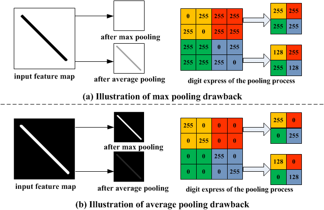
• Max Pooling: For each window, the output is the maximum value in that window.
• Average Pooling: For each window, the output is the average of all values in that window.

Let's watch a video that explains and visualizes these two operations.

To summarize:

• Max Pooling is the most common type used in modern CNNs. It is effective at capturing the most prominent (highest activation) feature in a patch. This makes it robust to noise and helps preserve the strongest signals.
• Average Pooling provides a smoothed, more generalized summary of a region. It was more common in older architectures but is less used today for feature extraction, as it can dilute the signal from a strong but localized feature.

The image below provides a fantastic visual and numerical comparison of the two pooling types.

For a more formal definition and another clear numerical example, please review the following text.

3. The Effect of Pooling on Spatial Dimensions

Now, let's focus on the primary effect of pooling: changing the dimensions of the feature maps.

A pooling layer is defined by its window size (or pool size) and its stride. Just like in a convolutional layer, the window size determines the area being summarized, and the stride determines how many pixels the window moves at each step.

A very common configuration for a pooling layer is a 2x2 window with a stride of 2. This setup has a simple and predictable effect: it halves the height and width of the input feature map. For example, a 32x32 feature map becomes a 16x16 feature map. This aggressively downsamples the representation.

But what about the depth (the number of channels)? This is a crucial point of distinction from convolutional layers. A pooling operation is applied independently to each channel. It does not mix information across channels. Therefore, the number of output channels is always the same as the number of input channels.

Let's look at the VGG-16 architecture, a classic CNN, to see this in practice.

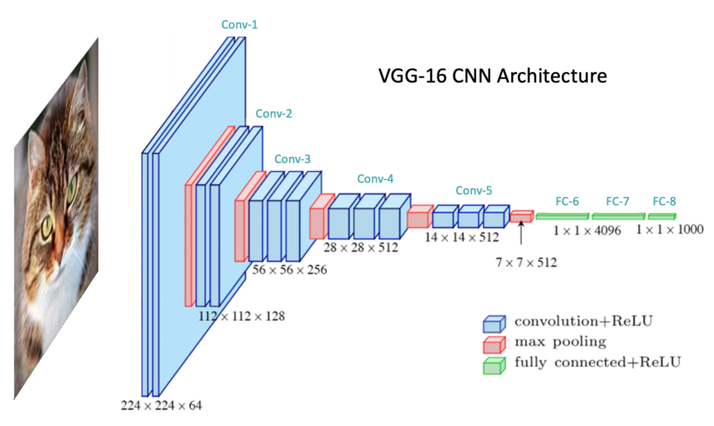
To confirm this behavior, watch this short clip that debugs a tensor as it passes through a max pooling layer.

Finally, the following reading explicitly states this rule about channels and summarizes the key aspects of pooling.

Conclusion

In this lesson, you've learned about the role and function of pooling layers, the essential counterpart to convolutional layers in a CNN. While convolutions extract features, pooling layers summarize them, making the network more efficient and robust.

Key Takeaways:

• The primary functions of pooling are to reduce spatial dimensions (downsampling), decrease computational cost, and introduce a degree of translational invariance.
• Max pooling, which selects the maximum value in a window, is the most common type and is effective at preserving the strongest features.
• Average pooling computes the mean of values in a window, which provides a more smoothed summary.
• A pooling layer's operation is governed by its window size and stride. A 2x2 window with a stride of 2 is a common choice that halves the height and width of the feature map.
• Crucially, pooling operates independently on each channel, meaning the depth of the feature map remains unchanged after a pooling operation.

Now that you understand the two fundamental building blocks of a CNN—Conv2d and MaxPool2d—you are ready to put them together. In the next lesson, you will define your first complete CNN architecture in PyTorch and use it for an image classification task.