Model Serving Strategies and Architectural Tradeoffs

Introduction

Welcome to our next lesson. In our previous discussion, we established the foundational MLOps principles for creating a reproducible and manageable machine learning model. We walked through the process of taking experimental code and data, tracking the experiment, versioning all assets (code, data, model), and finally storing the validated model artifact in a central model registry. A registered model is a governed, production-ready asset, but it is not yet delivering value. The crucial next step is to make its predictive power available to applications and users.

This lesson focuses on model serving, which is the process of deploying a machine learning model to a production environment so it can receive input data and return predictions. We will explore the primary strategies for serving models, centered around the fundamental tradeoff between generating predictions in large batches versus on-demand. You will learn to describe these strategies, analyze their architectural characteristics, and evaluate the tradeoffs in terms of latency, throughput, cost, and operational complexity. This will bridge the gap between a static model artifact and a live, value-generating AI system.

The Model Serving Landscape

Before diving into specific architectures, it's useful to build a conceptual map of the model serving landscape. The strategy you choose depends on two key dimensions: when the predictions are needed (Model Prediction) and how frequently the model is updated (Model Learning).

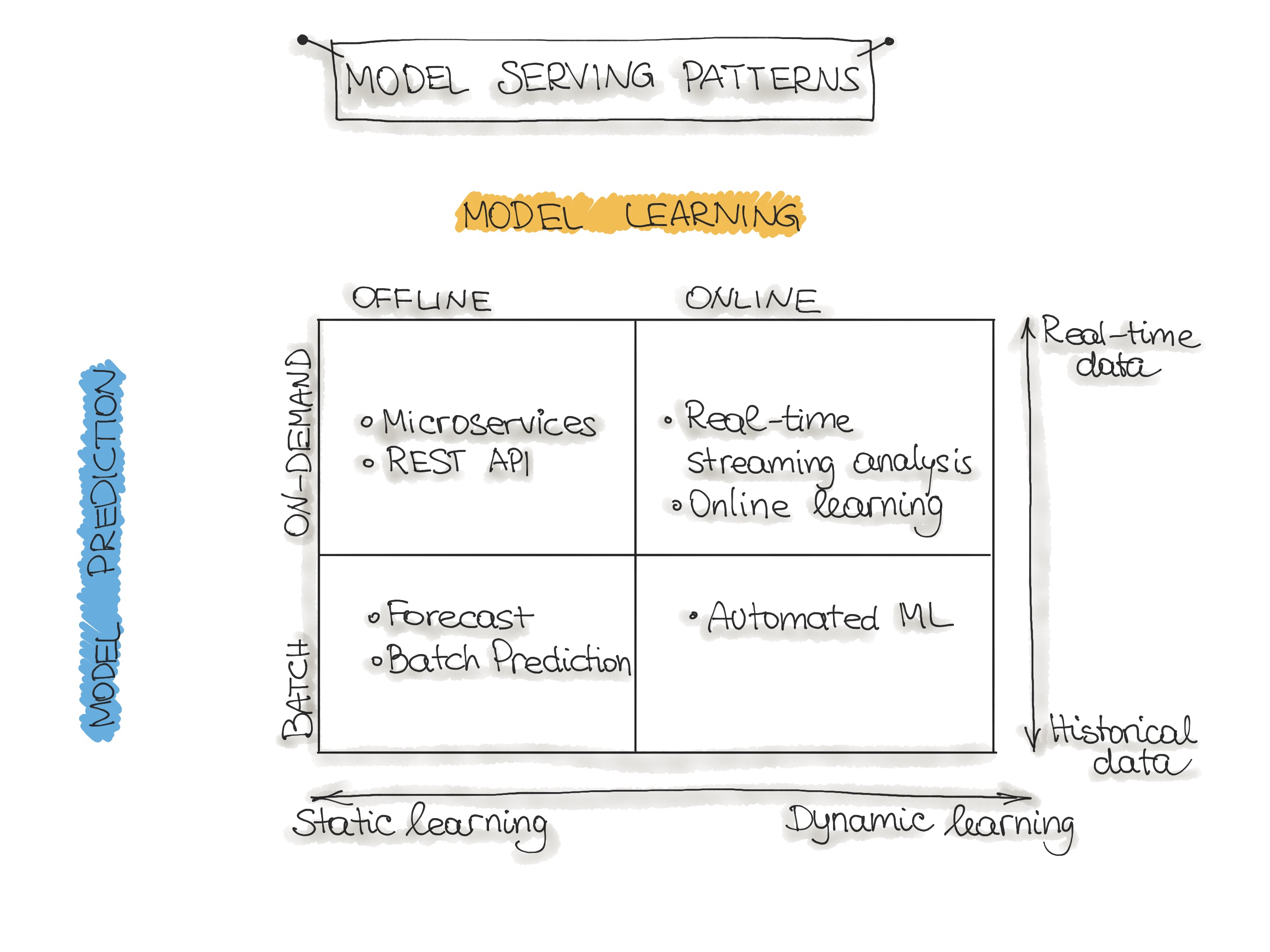
This 2x2 matrix provides a clear framework:

• Offline Learning / Batch Prediction: This is the most traditional pattern. A model is trained on a static, historical dataset and then used to score a large batch of new data on a schedule. Think of generating daily sales forecasts.
• Offline Learning / On-Demand Prediction: This is the most common pattern for interactive applications. A model is trained offline, but it's deployed as a live service (e.g., an API) to provide predictions instantly upon request. A real-time fraud detection system is a classic example.
• Online Learning / On-Demand Prediction: This is a more advanced pattern where the model not only serves predictions in real-time but also learns continuously from the stream of incoming data. This is suitable for highly dynamic environments, like ad-tech or content ranking.
• Online Learning / Batch Prediction: This is a less common pattern, but you can think of it as "Automated ML" where a system continuously retrains a model on new batches of data and then uses that updated model for batch predictions.

A crucial point of clarity is the term "real-time ML." It's often used ambiguously. For our purposes, we will make a sharp distinction.

With this framework in mind, let's explore the two dominant prediction strategies: batch and on-demand (real-time inference).

Strategy 1: Batch Prediction

In the batch prediction (or offline prediction) pattern, the application does not call a model directly. Instead, a separate process runs on a schedule (e.g., every hour or once a day), applies the model to a large volume of data, and saves the predictions to a database or data warehouse. Applications can then query these pre-computed results with very low latency.

Architectural Characteristics:

• Trigger: Scheduled, not event-driven. Orchestration tools like Apache Airflow or simple cron jobs are common.
• Data Scope: Operates on large, bounded datasets (e.g., "all transactions from yesterday," "the entire customer list").
• Performance: Optimized for high throughput (processing many records efficiently) rather than low latency. The time to generate a single prediction is not critical, but the time to process the entire batch is.
• Serving: The "serving" layer is often just a fast key-value store or a database table where an application can look up a prediction for a given ID.

Case Study: A Content Recommendation Engine

A common application of batch prediction is pre-generating recommendations. Instead of calculating what to recommend to a user at the exact moment they load a webpage, a system can do this work ahead of time.

Architectural Tradeoffs:

• Pros:
  • High Throughput: Can efficiently process massive amounts of data using scalable compute frameworks like Apache Spark.
  • Cost-Effective: Can use cheaper, ephemeral compute resources that only run when the batch job is active.
  • Decoupled: The prediction-generating process is completely separate from the user-facing application, reducing complexity in the application itself.
• Cons:
  • High Latency (Data Freshness): Predictions are not fresh. If the batch job runs daily, the predictions are based on data that is up to 24 hours old. This is unsuitable for use cases that require reacting to immediate events.

Strategy 2: Real-Time Inference

In the real-time inference (or online prediction) pattern, the model is deployed as a persistent, long-running service. Applications make direct requests to this service—typically via an API—and receive a prediction in milliseconds. This pattern is essential for any interactive use case where an immediate decision is required.

Architectural Characteristics:

• Trigger: Event-driven. An application makes a request (e.g., an HTTP POST request) to a model endpoint.
• Data Scope: Operates on single data points or small mini-batches provided in the request payload.
• Performance: Optimized for low latency. The primary goal is to return a prediction as quickly as possible, often within a strict service-level agreement (SLA) of 50-200ms.
• Serving: Involves deploying the model in a way that it can listen for and respond to network requests.

The choice of how to deploy this live service involves significant architectural tradeoffs. Given your background in systems, you'll recognize these patterns as variations on common microservice design principles.

Let's summarize the patterns from the reading:

1. Embedded Models: The model is a library or object within the application itself. This offers the lowest possible latency but creates tight coupling, making independent updates to the model difficult.
2. Sidecar Pattern: The model runs in a separate container alongside the application container in the same pod (in a Kubernetes context). This decouples the model from the application logic while maintaining low-latency communication over the local network.
3. Dedicated Model Servers: The model is deployed to specialized, centralized infrastructure (e.g., KServe, TensorFlow Serving, Amazon SageMaker Endpoints). This offers the most flexibility for independent scaling, A/B testing, and using specialized hardware like GPUs, but introduces network latency and additional operational overhead.

Case Study: Real-Time Fraud Detection

The canonical example for real-time inference is fraud detection during a financial transaction. A decision must be made in milliseconds, before the transaction is approved.

The cloud-native implementation of such a system often involves a combination of services, as shown in the AWS Summit presentation.

Strategy 3: Hybrid Architectures

Sometimes, neither pure batch nor pure real-time is sufficient. A hybrid approach may be needed to balance the need for comprehensive historical data with low-latency updates. The Lambda Architecture is a well-known design pattern for this.

The architecture consists of three layers:

1. Batch Layer: This is the familiar batch prediction system. It ingests all data and periodically re-computes a comprehensive set of results, or "batch views." This provides a complete and accurate, but not entirely fresh, picture.
2. Speed Layer (or Streaming Layer): This layer processes data streams in real-time. It computes results for only the most recent data, compensating for the high latency of the batch layer. Its results are less comprehensive but extremely fresh.
3. Serving Layer: This layer responds to user queries by merging the results from the batch view and the speed layer to provide a unified, up-to-date answer.

A recommendation engine is a great example. A daily batch job might compute recommendations based on a user's entire history (Batch Layer). A streaming process then updates these recommendations based on what the user is clicking on in their current session (Speed Layer). The final recommendations shown to the user are a combination of both.

Conclusion

In this lesson, we explored the critical step of deploying a trained model into a production environment. We have moved from a static artifact in a registry to a dynamic system that generates predictions.

Here are the key takeaways on model serving strategies:

• Serving is about tradeoffs: The central decision is between batch prediction (high throughput, high latency for freshness) and real-time inference (low latency, high operational complexity).
• Batch prediction is ideal for non-interactive use cases where predictions can be pre-computed on a schedule, like generating daily reports or propensity scores for a marketing campaign.
• Real-time inference is essential for interactive applications that need immediate predictions, like fraud detection. The implementation can range from simple embedded models to decoupled sidecars to powerful dedicated model servers, each with different implications for latency, scalability, and coupling.
• Hybrid patterns, like the Lambda Architecture, provide a blueprint for combining the comprehensive accuracy of batch processing with the low-latency updates of stream processing.
• It's crucial to distinguish real-time inference (using a static model for fast predictions) from online learning (continuously updating the model itself), with the former being far more common in production systems.

You now have a model deployed and serving predictions. But how do you know it's still performing well a week, or a month, after deployment? The world is not static, and the data patterns your model sees in production may change. In our next lesson, we will address this by exploring the concepts of data drift and model drift and the critical importance of production monitoring.