Understanding Data Drift, Model Drift, and Production Monitoring

Introduction

In our last lesson, we successfully navigated the process of deploying a trained model into a production environment, transforming it from a static artifact into a live service that delivers predictions. We established that the primary architectural decision revolves around the tradeoff between batch prediction and real-time inference. However, deploying a model is not the final step; it is the beginning of its operational lifecycle. A fundamental, and often unspoken, assumption in machine learning is that the future will resemble the past—that the patterns the model learned from historical data will continue to hold true for new, unseen data.

This lesson confronts the reality that this assumption is frequently violated. The world is not static; user behaviors evolve, economic conditions shift, and data collection systems change. This phenomenon, known as drift, can silently and steadily degrade a model's performance, turning a once-accurate system into a source of costly errors. We will formally define the two primary types of drift—data drift and concept drift—and explore their theoretical underpinnings. Most importantly, you will learn why production monitoring is not just a best practice but a theoretical necessity for maintaining robust and reliable AI systems.

The Theory of Drift: When the World Changes

At its core, a supervised machine learning model learns to approximate the joint probability distribution of features $X$ and a target variable $y$, denoted as $P(X,y)$. This is the statistical "world" the model understands based on its training data at time $t_0$. The model's utility rests on the assumption that for any future time $t$, the distribution remains the same: $P_{t_0}(X,y)=P_t(X,y)$.

Drift occurs when this assumption breaks. The core theoretical insight is that this joint probability can be factored into two components using the chain rule of probability:

A change in either of these components leads to a different type of drift, each with distinct implications for the model.

Let's solidify these definitions:

• Data Drift (or Covariate Shift): This occurs when the distribution of the input features $X$ changes, but the underlying relationship between features and the target $y$ remains the same. Mathematically, $P_t(X)\ne P_{t_0}(X)$, while $P_t(y|X)=P_{t_0}(y|X)$.

  • Example: A loan approval model was trained on data from a specific country. The bank expands to a new country where average incomes and debt levels (the features) are different. The criteria for what constitutes a "good loan" (the concept) haven't changed, but the input data distribution has.

• Concept Drift (or Real Drift): This is a more fundamental change where the statistical relationship between the input features and the target variable changes. The very meaning of the concept the model is trying to predict has shifted. Mathematically, $P_t(y|X)\ne P_{t_0}(y|X)$.

  • Example: In a spam detection model, the features of a "spam" email change over time. What was once characterized by certain keywords ("free," "viagra") is now characterized by new tactics (e.g., subtle phishing links, social engineering). The concept of "spam" itself has evolved.

The term model drift is often used colloquially to describe the observable degradation in a model's performance over time. This is almost always a symptom of underlying concept drift, as a change in $P(y|X)$ directly invalidates the function the model learned. Data drift can sometimes cause model drift, but not always. If the model is robust and has learned the true underlying relationship, it might generalize to new regions of the feature space. However, data drift is often a leading indicator that concept drift may also be occurring.

The Importance of Monitoring: Why Drift is a Production-Critical Issue

Ignoring drift is not an option for any production ML system. The consequences range from gradual erosion of business value to catastrophic failures.

As the video highlights, drift can be caused by two main factors:

1. Genuine Changes in the World: These are external factors that alter data patterns.

   • User Behavior: The COVID-19 pandemic dramatically shifted e-commerce patterns.
   • Economic Factors: Inflation or recession can change the criteria for creditworthiness.
   • Seasonality: A recommendation engine for clothing needs to adapt from summer to winter.
   • Adversarial Changes: Fraudsters and spammers constantly evolve their methods to evade detection models.

2. Data Integrity Issues: These are internal, system-level problems that manifest as drift.

   • Upstream Data Changes: A different team changes the schema of a source table without notification.
   • Pipeline Bugs: An error in a data processing job starts feeding null or incorrect values to the model.
   • Sensor Degradation: A physical sensor in an IoT device begins to fail, sending noisy data.

From a systems perspective, you can see that monitoring for drift is not just about model accuracy; it's a form of end-to-end integrity checking for your entire data pipeline.

Detecting Drift: The Practice of Monitoring

Now that we have established the "what" and "why" of drift, we turn to the "how." How do we algorithmically detect that a distribution has changed? The approach depends entirely on whether we have access to ground truth labels in a timely manner.

1. Detecting Concept Drift via Performance Monitoring

If you have access to ground truth labels for the predictions your model is making, you can directly measure the impact of drift. This is the most straightforward approach.

• Method: You continuously calculate your model's key performance indicators (KPIs) like accuracy, precision, recall, F1-score, or MSE on recent production data. You then compare these live metrics against the metrics from a reference window (e.g., the validation set or an earlier period of production).
• Signal: A statistically significant drop in performance is a strong signal that concept drift has occurred and is impacting your model (i.e., model drift).
• Challenge: The main limitation is label latency. For many real-world problems (e.g., predicting customer churn, loan defaults), the ground truth is only known weeks or months later. By then, the damage from the degraded model is already done. In such cases, you may need to rely on proxy metrics, as mentioned in the article you read.

2. Detecting Data Drift via Distribution Monitoring

When labels are delayed or unavailable, the primary strategy is to monitor for data drift. The logic is simple: while we can't observe $P_t(y|X)$ changing, we can always observe if $P_t(X)$ is changing, because we have the input features for every prediction request.

This involves comparing the statistical distribution of the incoming production data against a baseline or reference distribution (typically the training data).

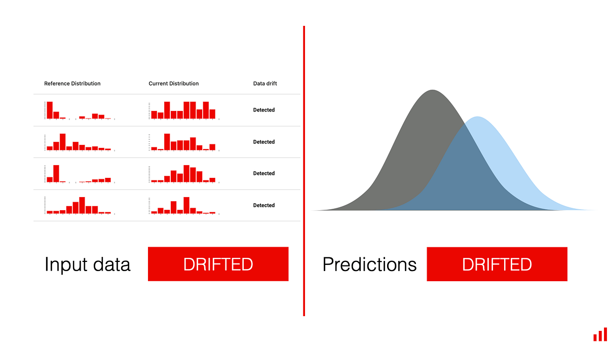
A variety of statistical tests and metrics are used to quantify the difference between two distributions.

To recap the key detection methods:

• Kolmogorov-Smirnov (K-S) Test: A non-parametric test that compares the cumulative distribution functions of two samples. It's powerful for detecting changes in both location and shape of a continuous distribution.
• Population Stability Index (PSI): Widely used in finance, it bins continuous data into histograms and computes a single number representing the difference in the percentage of observations in each bin between two samples.
• Chi-Squared Test: The standard method for comparing the distributions of categorical features.
• Autoencoder-based Reconstruction Error: A sophisticated multivariate method. You train an autoencoder on the reference data. When new data comes in, you pass it through the autoencoder. If the new data is "out-of-distribution," the autoencoder will struggle to reconstruct it, leading to a higher reconstruction error, which signals drift.

The MLOps Loop: From Detection to Action

Identifying drift is only half the battle. The ultimate goal of a production monitoring system is to serve as a trigger for automated action, closing the MLOps loop.

The process is as follows:

1. Monitor: A monitoring service continuously computes drift metrics (e.g., PSI on key features) or performance metrics (e.g., accuracy) on production data.
2. Alert: When a metric crosses a pre-defined threshold, the system sends an alert (e.g., to a human operator, or directly to an automation system).
3. Analyze: An automated process or a data scientist investigates the alert. Is it a data pipeline bug? Or is it genuine concept drift? Explainability tools can be used here to pinpoint which features are drifting and how they are impacting predictions.
4. Act: Based on the analysis, an action is taken. This could be:
   • Fixing a bug in the data pipeline.
   • Triggering an automated retraining pipeline to create a new model version using the latest data.
   • Rolling back to a previous model version.
   • Taking the model offline and falling back to a rule-based system.

Conclusion

In this lesson, we have demystified one of the most critical challenges in production machine learning: model and data drift. We have established that the "stationary world" is a myth, and that robust AI systems must be designed with the explicit assumption that the environment will change.

Here are the key theoretical and practical takeaways:

• Drift is a change in data's statistical properties over time. It is formally defined as a change in the joint probability distribution $P(X,y)$.
• Data Drift is a change in the input distribution $P(X)$, while Concept Drift is a change in the input-output relationship $P(y|X)$. Model performance degradation, or Model Drift, is typically a symptom of concept drift.
• Production Monitoring is essential to detect drift before it causes significant harm. It provides a crucial feedback loop for the health of your ML system.
• Detection strategies are twofold: If ground truth labels are available, performance monitoring directly measures the impact of concept drift. If not, data distribution monitoring uses statistical tests (like K-S, PSI) on input features to detect data drift, which serves as a powerful leading indicator.
• The goal of monitoring is automated action. A mature MLOps system uses drift detection as a trigger to initiate remediation, most commonly by launching an automated retraining pipeline.

We have now covered the full lifecycle of an MLOps pipeline: from experiment tracking and versioning, to model deployment and serving, and finally to production monitoring and maintenance. In our final lesson for this module, we will synthesize this knowledge by contrasting the Continuous Integration/Continuous Deployment (CI/CD) paradigm for traditional software with the unique challenges and requirements of CI/CD for ML systems, where code, models, and data all must be managed in lockstep.