Gradient Descent for Linear Regression in Python

Introduction

In our previous lesson, we accomplished a significant theoretical step: deriving the gradient descent update rule, ${\mathbf{w}}_{t+1}={\mathbf{w}}_t-\alpha \nabla L({\mathbf{w}}_t)$, directly from a first-order Taylor approximation. We established that this isn't just an intuitive idea of "walking downhill," but a mathematically grounded method for finding the direction of steepest local descent on a loss surface.

Today, we transition from this abstract derivation to concrete implementation. Our goal is to bring the gradient descent algorithm to life by applying it to solve a foundational problem in machine learning: linear regression. You will implement the entire algorithm from scratch in Python, translating the mathematical components—the model, the loss function, and the gradient—into functional code. This lesson will bridge the gap between the "why" of the theory and the "how" of a practical, working optimization routine.

The Problem Setup: Linear Regression and MSE

Before we can implement the update rule, we must define the three specific components it requires:

1. The Model: A function that makes predictions.
2. The Loss Function: A function that measures the error of those predictions.
3. The Gradient: The derivative of the loss with respect to the model's parameters.

For this task, we will use the linear regression model. In its general, vectorized form, the model's prediction $\hat{\mathbf{y}}$ for a set of N examples with P features is:

$$\hat{\mathbf{y}}=\mathbf{Xw}$$

Here, $\mathbf{X}$ is the $N\times (P+1)$ design matrix (with a column of ones prepended for the bias term), and $\mathbf{w}$ is the $(P+1)\times 1$ vector of weights.

The most common loss function for regression is the Mean Squared Error (MSE), which measures the average squared difference between the true values $\mathbf{y}$ and our predictions $\hat{\mathbf{y}}$.

The MSE loss function, $L(\mathbf{w})$, is formally written as:

$$L(\mathbf{w})=\frac{1}{N}\sum _{i=1}^N(y_i-{\hat{y}}_i{)}^2=\frac{1}{N}\sum _{i=1}^N(y_i-{\mathbf{x}}_i^T\mathbf{w}{)}^2$$

where ${\mathbf{x}}_i^T$ is the i-th row of the design matrix $\mathbf{X}$.

Deriving the Gradient of the MSE Loss

Our update rule, ${\mathbf{w}}_{t+1}={\mathbf{w}}_t-\alpha \nabla L({\mathbf{w}}_t)$, requires the gradient of the MSE loss function, $\nabla L(\mathbf{w})$. This gradient is a vector containing the partial derivative of the loss with respect to each weight $w_j$.

My question for you is: Given your experience with matrix calculus, can you derive the gradient of the MSE loss function, ${\nabla }_{\mathbf{w}}L(\mathbf{w})$, with respect to the entire weight vector $\mathbf{w}$?

Hint: It's often easier to start with the vectorized form of the loss, $L(\mathbf{w})=\frac{1}{N}(\mathbf{y}-\mathbf{Xw}{)}^T(\mathbf{y}-\mathbf{Xw})$, and apply the rules of matrix differentiation.

Let's work through it.

1. Expand the expression: $L(\mathbf{w})=\frac{1}{N}({\mathbf{y}}^T\mathbf{y}-2{\mathbf{y}}^T\mathbf{Xw}+{\mathbf{w}}^T{\mathbf{X}}^T\mathbf{Xw})$.
2. Take the derivative with respect to $\mathbf{w}$:
   • ${\nabla }_{\mathbf{w}}({\mathbf{y}}^T\mathbf{y})=0$ (no $\mathbf{w}$ term).
   • ${\nabla }_{\mathbf{w}}(-2{\mathbf{y}}^T\mathbf{Xw})=-2{\mathbf{X}}^T\mathbf{y}$.
   • ${\nabla }_{\mathbf{w}}({\mathbf{w}}^T{\mathbf{X}}^T\mathbf{Xw})=2{\mathbf{X}}^T\mathbf{Xw}$ (since ${\mathbf{X}}^T\mathbf{X}$ is symmetric).
3. Combine the terms: $${\nabla }_{\mathbf{w}}L(\mathbf{w})=\frac{1}{N}(-2{\mathbf{X}}^T\mathbf{y}+2{\mathbf{X}}^T\mathbf{Xw})=\frac{2}{N}{\mathbf{X}}^T(\mathbf{Xw}-\mathbf{y})$$

This final expression is the gradient we need. It's computationally elegant because it relies on matrix-vector multiplications, which are highly optimized in libraries like NumPy.

The following resources walk through this derivation in detail, either for individual parameters m and b or in a vectorized form.

Implementation From Scratch

Now we have all the pieces to build our regressor. We will structure this in a Python class for clarity and reusability. An efficient implementation will use NumPy for vectorized operations, avoiding explicit for loops over the data, which is crucial for performance—a topic that aligns with your interest in systems engineering.

The video below by Aladdin Persson provides an excellent, clean, and vectorized implementation that we will use as a guide.

Following this structure, let's outline the code.

1. Generating Data and Setting up the Class

First, let's create some synthetic data to test our algorithm and define the skeleton of our LinearRegression class.

import numpy as np
import matplotlib.pyplot as plt




# Generate some synthetic data
X = 2 * np.random.rand(100, 1)
y = 4 + 3 * X + np.random.randn(100, 1) # y = 4 + 3x + noise




# Plot the data
plt.scatter(X, y)
plt.xlabel("Feature (x)")
plt.ylabel("Target (y)")
plt.title("Synthetic Data for Linear Regression")
plt.show()

class LinearRegression:
    def __init__(self, learning_rate=0.01, n_iterations=1000):
        self.learning_rate = learning_rate
        self.n_iterations = n_iterations
        self.weights = None
        self.cost_history = []

    def fit(self, X, y):



        # Implementation to follow
        pass

    def predict(self, X):



        # Implementation to follow
        pass

2. The fit Method: The Heart of Gradient Descent

The fit method will contain the core gradient descent loop.

1. Prepare the data: We add a column of ones to X to account for the bias term w_0. This is the "bias trick."
2. Initialize weights: We'll initialize the weights vector $\mathbf{w}$ with small random numbers.
3. Iterate: Loop for n_iterations:
   a. Calculate predictions $\hat{\mathbf{y}}={\mathbf{X}}_{\mathbf{b}}\mathbf{w}$.
   b. Calculate the gradient $\nabla L=\frac{2}{N}{{\mathbf{X}}_{\mathbf{b}}}^T(\hat{\mathbf{y}}-\mathbf{y})$.
   c. Update the weights $\mathbf{w}\leftarrow \mathbf{w}-\alpha \nabla L$.

class LinearRegression:
    def __init__(self, learning_rate=0.01, n_iterations=1000):
        self.learning_rate = learning_rate
        self.n_iterations = n_iterations
        self.weights = None
        self.cost_history = []

    def fit(self, X, y):



        # 1. Prepare data (add bias term)
        n_samples, n_features = X.shape
        X_b = np.c_[np.ones((n_samples, 1)), X]  # Add x0 = 1 to each instance




        # 2. Initialize weights
        self.weights = np.random.randn(n_features + 1, 1)




        # 3. Gradient Descent loop
        for i in range(self.n_iterations):



            # a. Calculate predictions
            y_predicted = X_b.dot(self.weights)




            # b. Calculate gradient
            gradients = (2 / n_samples) * X_b.T.dot(y_predicted - y)




            # c. Update weights
            self.weights = self.weights - self.learning_rate * gradients
            



            # Optional: store cost to visualize
            cost = np.mean((y_predicted - y)**2)
            self.cost_history.append(cost)
            
        return self

    def predict(self, X):
        X_b = np.c_[np.ones((X.shape[0], 1)), X]
        return X_b.dot(self.weights)

3. Training and Visualizing the Result

Now we can use our class to train the model and see the result.

# Instantiate and train the model
regressor = LinearRegression(learning_rate=0.1, n_iterations=1000)
regressor.fit(X, y)

print("Final weights (w0, w1):", regressor.weights.flatten())




# Plot the regression line
X_new = np.array([[0], [2]])
y_predict = regressor.predict(X_new)

plt.scatter(X, y, label="Data points")
plt.plot(X_new, y_predict, "r-", label="Prediction")
plt.xlabel("Feature (x)")
plt.ylabel("Target (y)")
plt.title("Linear Regression with Gradient Descent")
plt.legend()
plt.show()




# Plot the cost history
plt.plot(range(regressor.n_iterations), regressor.cost_history)
plt.xlabel("Iteration")
plt.ylabel("Cost (MSE)")
plt.title("Cost Function Convergence")
plt.show()

You should see that the final weights are close to our true parameters (4 and 3) and that the cost function decreases steadily over iterations, indicating that our optimizer is working correctly.

The Role of the Learning Rate

The hyperparameter $\alpha$, our learning rate, is critical. It controls the size of each step we take down the loss surface.

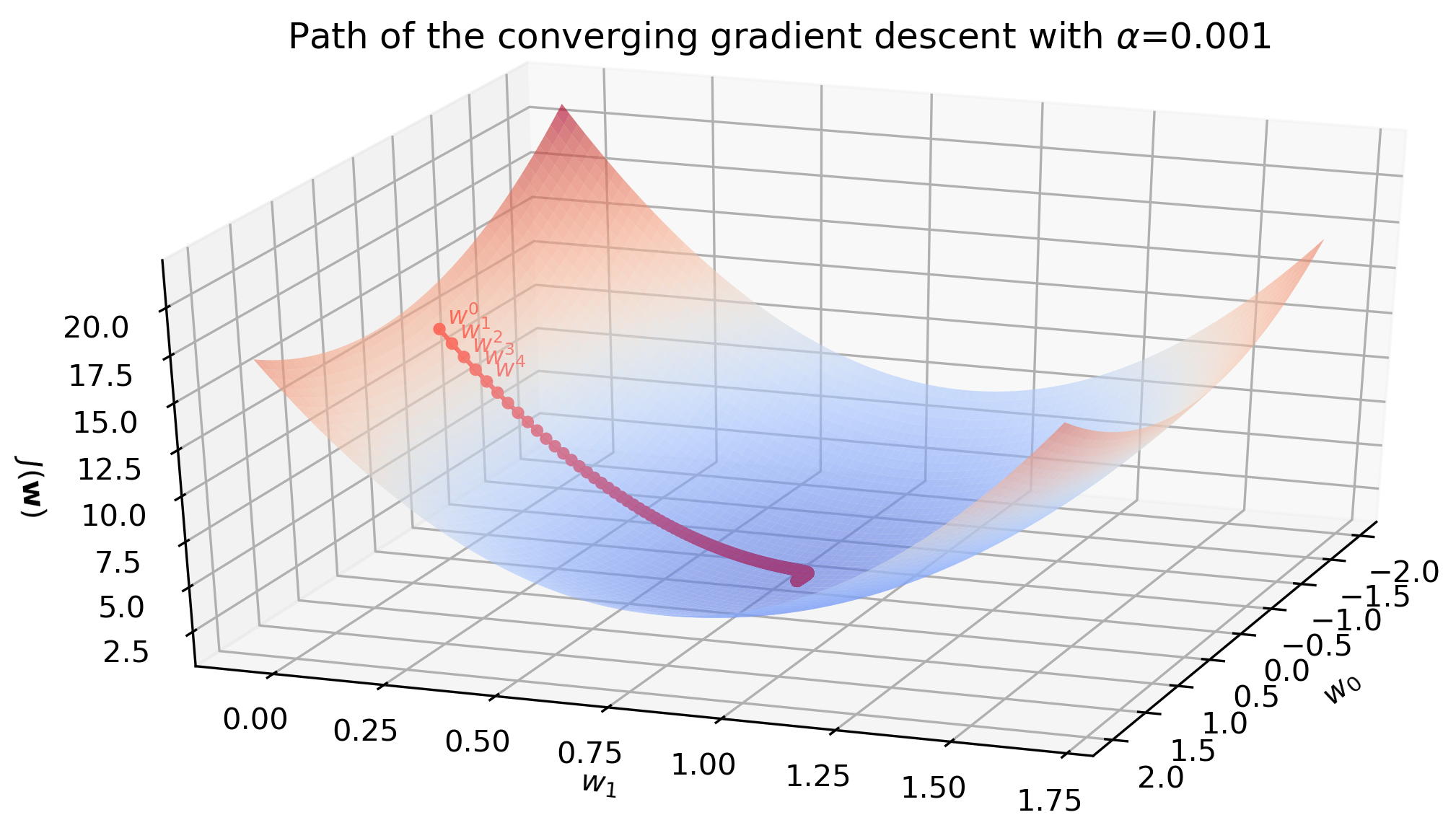
If $\alpha$ is too small, convergence will be very slow. If it's too large, the updates will overshoot the minimum, causing the loss to oscillate or even diverge catastrophically.

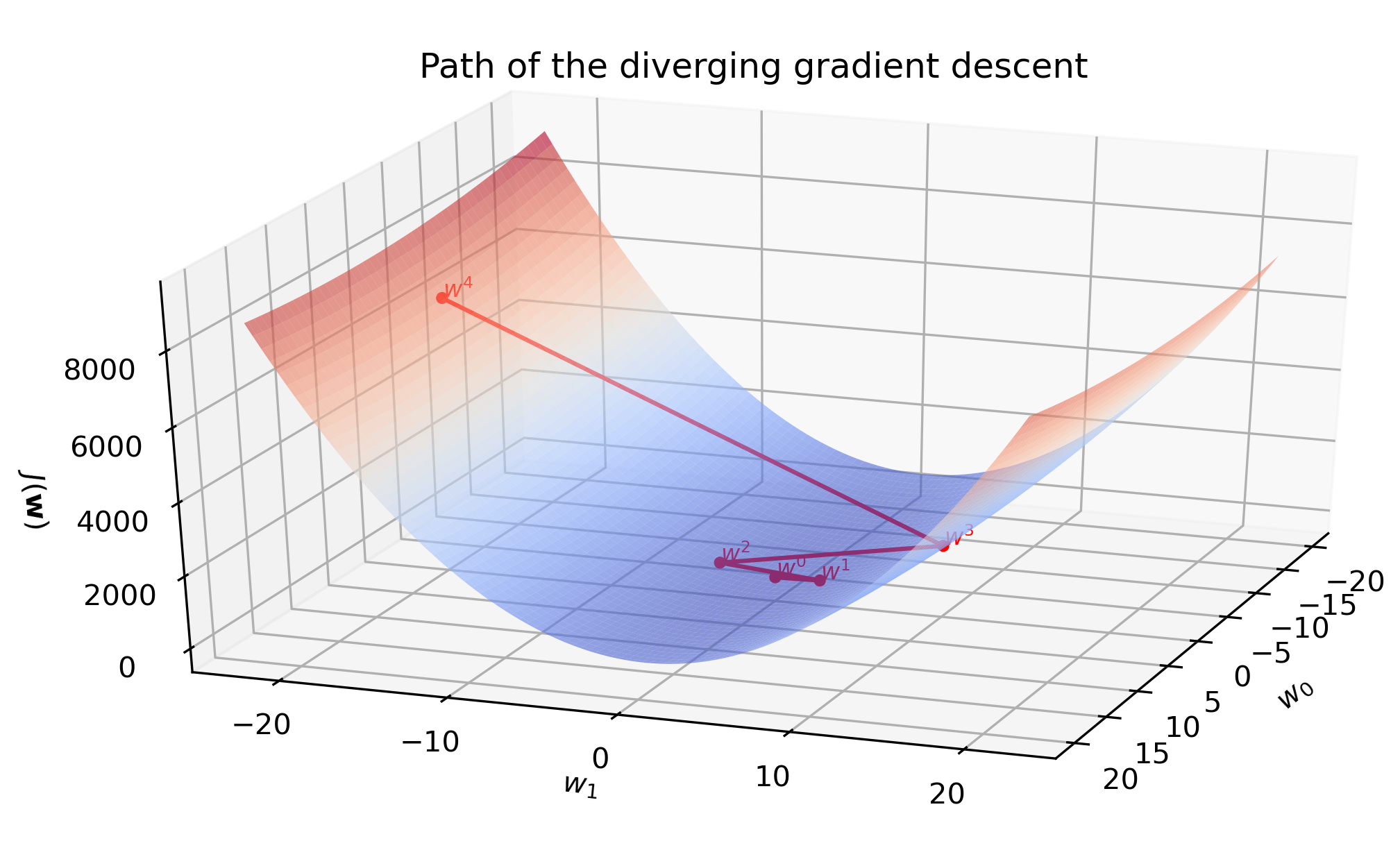
Try running the code above with different learning_rate values (e.g., 0.001, 0.5, 1.0) and observe the effect on the cost history plot. This hands-on experimentation is key to building intuition.

Conclusion

In this lesson, we successfully translated the theory of gradient descent into a practical, from-scratch implementation for linear regression. We defined our model and loss function, derived the necessary gradient using matrix calculus, and built a vectorized Python implementation that efficiently finds the optimal model parameters.

Key Takeaways:

• Theory to Practice: The abstract update rule ${\mathbf{w}}_{t+1}={\mathbf{w}}_t-\alpha \nabla L({\mathbf{w}}_t)$ is made concrete by supplying a specific model ($\hat{\mathbf{y}}=\mathbf{Xw}$) and loss (MSE).
• Vectorization is Power: Implementing the gradient calculation with matrix operations ($\frac{2}{N}{\mathbf{X}}^T(\mathbf{Xw}-\mathbf{y})$) is far more efficient than looping through data points, a key principle in high-performance scientific computing.
• The Algorithm in Action: The core of gradient descent is an iterative loop: predict, calculate gradient, and update weights.
• Hyperparameter Sensitivity: The learning rate $\alpha$ is a critical knob that dictates the stability and speed of convergence.

Preview of the Next Lesson:

We've seen firsthand how changing the learning rate can drastically affect our model's training. In our next lesson, we will formalize this exploration. We will delve into methods for diagnosing the effects of the learning rate, discuss common strategies for choosing a good value, and introduce the concept of learning rate schedules.