Gradient Descent: The Taylor Expansion Approach

Recommended resources

The freely available resources this lesson will direct you to.

Introduction

In our last lesson, we established the critical trade-off between direct and iterative optimization methods. We saw that while the Normal Equation for Ordinary Least Squares provides a "one-shot" exact solution, its computational cost, particularly the $O (P^{3})$ complexity of matrix inversion, makes it impractical for the high-dimensional problems typical in modern AI. This realization motivates our turn to iterative methods, with Gradient Descent as the cornerstone.

Today, we transition from the why to the how. Our objective is to derive the famous gradient descent update rule from first principles. We will see that this algorithm is not just an intuitive idea of "walking downhill," but a direct mathematical consequence of approximating a complex loss function with a simple local model. The central tool for this derivation will be the Taylor series, a powerful concept from calculus that allows us to understand a function's behavior in the neighborhood of a point.

The Power of Local Approximation: Taylor Series

Imagine our loss function $L (w)$ is a complex, high-dimensional landscape. We are standing at a point $w_{t}$ and want to take a small step to a new point $w_{t + 1}$ that is lower. The landscape is too complicated to understand globally, but we can create a simplified local map around our current position.

The most straightforward local map we can create is a linear one. Think of it as laying a flat tangent plane on the curved surface of the loss function at our current point.

My first question for you is: If you wanted to create the best possible linear approximation for a function $L (w)$ at a specific point $w_{0}$ , what two properties must your line share with the function at that exact point?

Think about what makes an approximation "good" at a single point. It should not only pass through the same point but also move in the same direction. This means the line and the function must share:

The same value: The line's value at $w_{0}$ must be $L (w_{0})$ .
The same slope: The line's derivative at $w_{0}$ must be $L^{'} (w_{0})$ .

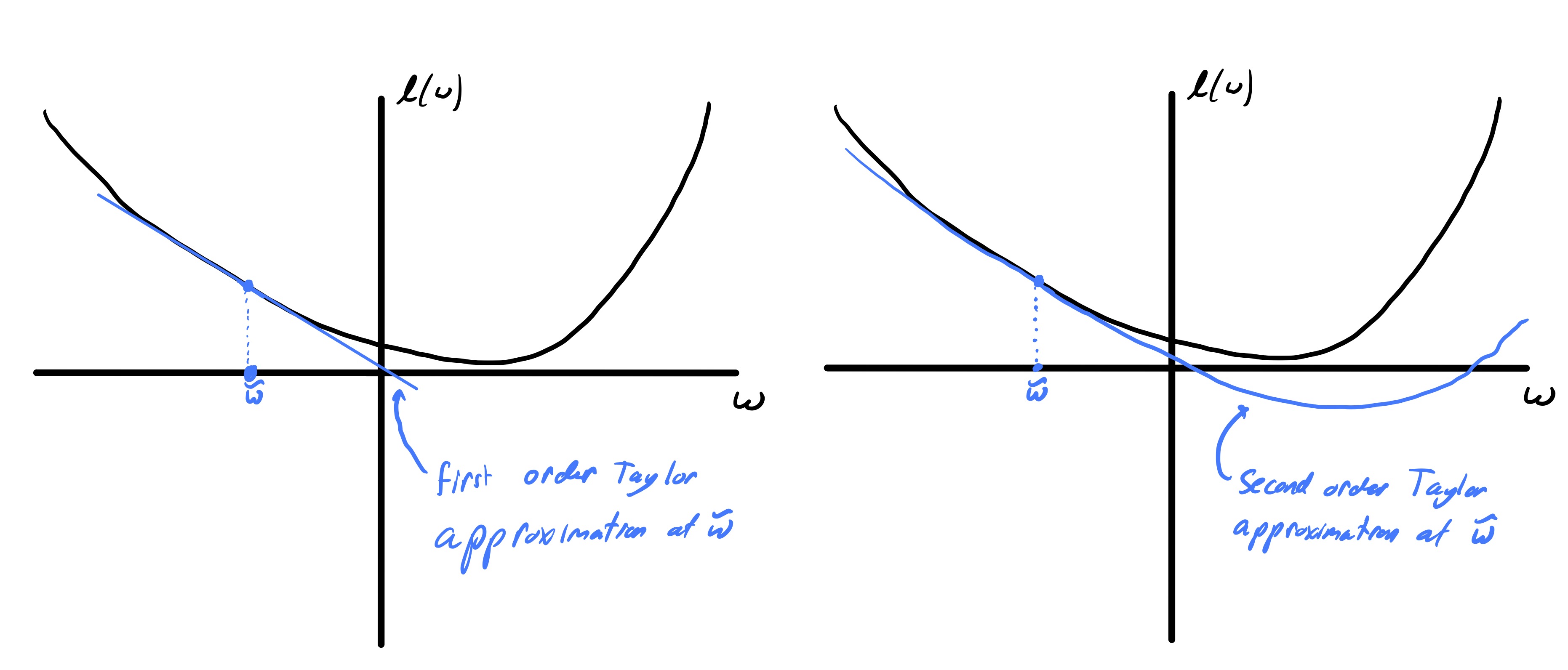
This is the fundamental insight behind a first-order Taylor approximation. It states that for a small step $Δ w$ , the value of the function at a new point $w_{0} + Δ w$ can be approximated by:

L (w_{0} + Δ w) \approx L (w_{0}) + L^{'} (w_{0}) Δ w

This equation essentially says, "The new value is the old value plus the rate of change times the size of the step." The following image beautifully illustrates this concept, comparing a linear (first-order) approximation to a quadratic (second-order) one.

A visual comparison of a first-order (linear) and second-order (quadratic) Taylor approximation of a function L(w) at a point w̃. The linear approximation is the tangent line at that point.

To build a strong intuition for how these approximations are constructed, the following video by 3Blue1Brown is an excellent resource. It masterfully explains the idea of building polynomial approximations by matching derivatives one by one.

Taylor series | Chapter 11, Essence of calculus

This video, "Taylor series" from the channel 3Blue1Brown, provides a beautiful and intuitive explanation of how to approximate functions with polynomials.

Watch the segments on the motivation for approximation and the step-by-step construction of a quadratic approximation for cos(x). Focus on how each term in the polynomial is chosen to match a derivative of the original function at a specific point.

Deriving the 1D Gradient Descent Update

Now, let's use this tool for our goal of optimization. We are at a point $w_{t}$ and want to choose a step, $Δ w$ , that takes us to a new point $w_{t + 1} = w_{t} + Δ w$ such that the loss decreases, i.e., $L (w_{t + 1}) < L (w_{t})$ .

Using our first-order Taylor approximation:

L (w_{t + 1}) = L (w_{t} + Δ w) \approx L (w_{t}) + L^{'} (w_{t}) Δ w

To make the loss decrease, we want the change in loss, $L (w_{t + 1}) - L (w_{t})$ , to be negative:

L (w_{t + 1}) - L (w_{t}) \approx L^{'} (w_{t}) Δ w < 0

This inequality is the heart of our derivation. We need to choose a step $Δ w$ that makes the product $L^{'} (w_{t}) Δ w$ negative.

Here is my second question for you: We have complete control over our step $Δ w$ . Given that the derivative $L^{'} (w_{t})$ at our current location is a fixed value (it could be positive or negative), how should we choose $Δ w$ to make the product $L^{'} (w_{t}) Δ w$ not just negative, but as negative as possible? This would ensure we are moving in the direction of steepest descent.

To make the product of two numbers as negative as possible, one should be positive and the other negative. Specifically, to minimize $A \cdot B$ where we control $B$ , we should choose $B$ to have the opposite sign of $A$ and a large magnitude. In our case, this means our step $Δ w$ should be proportional to the negative of the derivative $L^{'} (w_{t})$ .

We can write this relationship as:

Δ w = - α L^{'} (w_{t})

Here, $α$ (alpha) is a small, positive constant called the learning rate. It's our "proportionality constant" that controls the size of the step we take. It needs to be small enough to ensure that our linear approximation remains valid.

Substituting this choice of $Δ w$ back into our update rule gives us the celebrated gradient descent update rule for one dimension:

w_{t + 1} = w_{t} + Δ w = w_{t} - α L^{'} (w_{t})

Let's verify this choice. If we plug it into our approximation for the change in loss:

L (w_{t + 1}) - L (w_{t}) \approx L^{'} (w_{t}) \cdot (- α L^{'} (w_{t})) = - α (L^{'} (w_{t}))^{2}

Since $α > 0$ and $(L^{'} (w_{t}))^{2} \geq 0$ , the entire right-hand side is guaranteed to be less than or equal to zero. The loss will decrease as long as the derivative is non-zero.

The following resource provides a clear, step-by-step derivation of this exact logic.

9 Optimization with Gradient Descent – Machine Learning

This text by Prof. Phil Chodrow provides a concise mathematical derivation of gradient descent.

First, review the section on Taylor's Theorem for univariate functions to solidify the formal definition. Then, carefully study the section deriving the 1D update rule. Notice how it uses the Taylor approximation to show that the update \hat{w} \gets \hat{w} - \alpha \frac{dg(\hat{w})}{dw} is guaranteed to reduce the function value.

Generalizing to Multiple Dimensions

In machine learning, our loss function $L (w)$ almost always depends on a vector of many parameters $w \in R^{P}$ . The principles remain the same, but our calculus tools must be upgraded to their multivariable equivalents.

The derivative $L^{'} (w)$ becomes the gradient $\nabla L (w)$ . The gradient is a vector of all partial derivatives: $[\frac{\partial L}{\partial w _{1}}, \frac{\partial L}{\partial w _{2}}, \dots, \frac{\partial L}{\partial w _{P}}]^{T}$ . Geometrically, it points in the direction of the steepest ascent of the function.
The product $L^{'} (w) Δ w$ becomes the dot product $\nabla L (w)^{T} Δ w$ .

The multivariate first-order Taylor approximation is therefore:

L (w_{t} + Δ w) \approx L (w_{t}) + \nabla L (w_{t})^{T} Δ w

Our goal is the same: choose a step vector $Δ w$ to make the change in loss, $\nabla L (w_{t})^{T} Δ w$ , as negative as possible. From linear algebra, we know that the dot product of two vectors $a^{T} b$ is minimized when the vector $b$ points in the exact opposite direction of vector $a$ .

Therefore, the direction of steepest descent for $Δ w$ must be the direction of the negative gradient, $- \nabla L (w_{t})$ . We again introduce the learning rate $α$ to control the step size:

Δ w = - α \nabla L (w_{t})

This gives us the final, general form of the gradient descent update rule:

w_{t + 1} = w_{t} - α \nabla L (w_{t})

The logic is identical to the 1D case. By taking a small step in the direction opposite to the gradient, we are moving along the path of steepest local descent, ensuring our loss decreases with each iteration.

The following resources formalize this multivariate derivation. I encourage you to read the first one, and use the second one as a supplementary reference.

9 Optimization with Gradient Descent – Machine Learning

This is the same text as before, now extending the logic to multiple dimensions.

Read the sections on Gradients and Multivariate Gradient Descent. This will show you how the exact same logic we used for the 1D case applies in higher dimensions, with the derivative being replaced by the gradient and multiplication by the dot product.

Gradient Descent and Taylor Series

This video lecture from IIT Madras directly addresses the question of "why the negative derivative?" using Taylor series. While it focuses on the 1D case, the reasoning is presented very clearly and applies directly to our multivariable derivation.

Watch from the beginning where the question is posed, through the introduction and application of Taylor series, and finally to the conclusion where the choice of the negative derivative is justified.

Conclusion

We have successfully derived the gradient descent algorithm from the ground up. This process wasn't arbitrary; it was a logical consequence of applying a fundamental tool from calculus—the Taylor series—to the problem of optimization. By creating a simple linear model of our complex loss function at our current position, we could mathematically determine the direction of steepest descent.

Key Takeaways:

Local Approximation is Key: Gradient descent works by approximating the complex loss landscape with a simple linear function (a tangent plane) at the current point.
Taylor Series Provides the Tool: The first-order Taylor expansion gives us the mathematical form of this linear approximation.
Steepest Descent: To minimize the loss locally, we must move in the direction that makes our linear approximation decrease most rapidly. This direction is precisely the negative gradient, $- \nabla L (w)$ .
The Update Rule: The final update rule, $w_{t + 1} = w_{t} - α \nabla L (w_{t})$ , combines the direction of steepest descent with a small step size $α$ (the learning rate) to ensure the local approximation holds.

Preview of the Next Lesson:

With the "why" and "how" of gradient descent now firmly established in theory, our next step is to bring it to life. In the upcoming lesson, you will implement the gradient descent algorithm from scratch in Python. We will apply it to the linear regression problem, closing the loop and providing a practical, code-based understanding of the powerful theoretical concepts we derived today.