Understanding Learning Rate: Impact on Convergence

Introduction

In our last lesson, you successfully implemented gradient descent from scratch for linear regression. A key part of that exercise was experimenting with the learning_rate hyperparameter, where you likely observed that its value dramatically influences the training process. A small learning rate led to slow convergence, while a large one caused the cost to behave erratically or even diverge.

Today, we will formalize this empirical understanding. Our objective is to explain the fundamental role of the learning rate and equip you with the tools to diagnose its effects on convergence. We will move beyond simple intuition to explore the mathematical reasons for its behavior, connecting it back to the Taylor series approximation that underpins gradient descent and even to second-order information about the loss function's curvature. We will also touch upon the theoretical guarantees of convergence, a topic that should appeal to your interest in systems performance.

The Role of the Learning Rate

Let's start by revisiting the gradient descent update rule:

We use $\eta$ (eta) here for the learning rate, which is equivalent to the $\alpha$ we've used previously. It is a scalar hyperparameter that controls the magnitude of the step we take in the direction opposite to the gradient.

The gradient, $\nabla L({\mathbf{w}}_k)$, gives us the direction of steepest ascent on the loss surface. By moving in the opposite direction, we are performing the method of steepest descent. The learning rate, $\eta$, determines how far we travel in that direction.

To build a strong mental model, let's watch a brief video that visualizes this process and its connection to the mathematics we've discussed.

Diagnosing the Effects of the Learning Rate

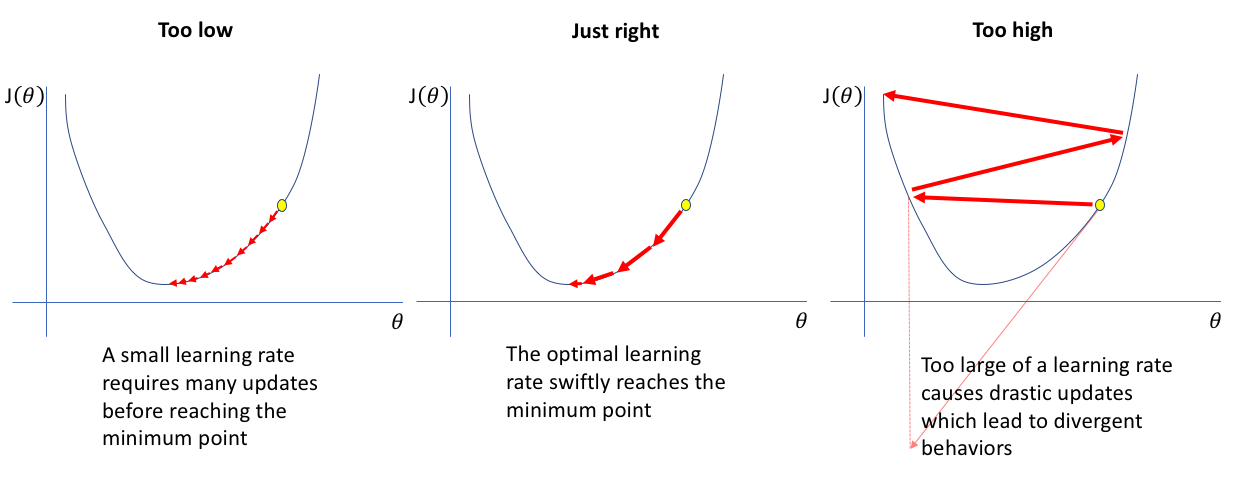
The video provides a clear visual intuition. A small $\eta$ results in tiny, cautious steps, leading to slow but steady progress. A large $\eta$ causes drastic updates that can overshoot the minimum, leading to oscillations or even divergence where the loss increases with each step. An optimal $\eta$ finds a balance, converging quickly and efficiently.

The image below, "The effect of learning rate," illustrates these three scenarios on a simple 1D quadratic loss function. The x-axis is the parameter value $\theta$, and the y-axis is the cost $J(\theta )$.

In practice, the most common way to diagnose the effect of the learning rate is by plotting the loss function value at each iteration, just as you did in the previous lesson's coding exercise.

These plots are your primary diagnostic tool:

• Loss diverges (goes up): Your learning rate is too high. Decrease it significantly (e.g., by a factor of 10).
• Loss oscillates wildly: Your learning rate is still too high. Decrease it (e.g., by a factor of 3).
• Loss decreases very slowly: Your learning rate is likely too low. Try increasing it (e.g., by a factor of 3).
• Loss decreases steadily: You're in a good range. You might experiment with slightly larger values to see if you can converge faster.

A Deeper Look: The Learning Rate and Curvature

Now, let's move to a first-principles explanation. Why does "too high" cause divergence? Recall that the gradient descent rule is derived from a first-order Taylor approximation:

This is a linear approximation of a likely non-linear function. This approximation is only accurate in a small neighborhood around ${\mathbf{w}}_k$. The learning rate $\eta$ controls the size of this neighborhood. If $\eta$ is too large, our step ${\mathbf{w}}_{k+1}-{\mathbf{w}}_k$ takes us so far from ${\mathbf{w}}_k$ that the linear approximation is no longer valid, and there is no guarantee that the loss will decrease.

We can gain even deeper insight by considering second-order information—the curvature of the loss function, captured by the Hessian matrix. For a simple 1D quadratic function $L(w)=\frac{1}{2}a{w}^2$, the first derivative (gradient) is $L^{\prime }(w)=aw$ and the second derivative (curvature) is $L^{\prime \prime }(w)=a$.

My question to you is: For this function $L(w)=\frac{1}{2}a{w}^2$, what would be the exact learning rate $\eta$ that allows you to reach the minimum at $w=0$ in a single step, starting from any point $w_k$?

Let's analyze this. The update rule is $w_{k+1}=w_k-\eta L^{\prime }(w_k)=w_k-\eta (a{w}_k)$. We want $w_{k+1}=0$.

For this to hold for any $w_k\ne 0$, we must have $1-\eta a=0$, which implies $\eta =1/a$.

This is a profound result: the optimal learning rate is the inverse of the function's curvature.

• High curvature (steep bowl, large $a$): We need a small learning rate.
• Low curvature (shallow bowl, small $a$): We need a large learning rate.

Since the loss surface of a neural network is highly complex and non-uniform, the local curvature changes from point to point. A fixed learning rate is therefore always a compromise.

This next reading explores this exact idea with concrete numerical examples.

Convergence Rate Analysis

For someone with your background in engineering and performance, it's not enough to know that it converges; you should also ask how fast it converges. This is the domain of optimization theory.

Under certain assumptions, we can provide a formal guarantee on the convergence rate of gradient descent. A key assumption is that the gradient of the loss function is L-Lipschitz continuous. This is a mathematical way of saying the function's curvature is bounded. Formally, there exists a constant $L>0$ such that for any two points $\mathbf{w}$ and $\mathbf{v}$:

If we set the learning rate $\eta \le 1/L$, we can guarantee that the loss will not increase. Furthermore, we can derive a bound on how quickly the algorithm converges. For a general non-convex function (the standard case in deep learning), it can be shown that after $t$ iterations, the minimum squared gradient norm found so far is bounded:

where $L(w_0)$ is the initial loss and $L^{\ast }$ is the minimum possible loss.

This is called a sublinear convergence rate. It means that to guarantee a solution with an error tolerance of $ϵ$ (i.e., $\Vert \nabla L{\Vert }^2\le ϵ$), we need $t=O(1/ϵ)$ iterations. This formalizes the diminishing returns you see in the loss plot: each additional "digit of accuracy" requires exponentially more work.

The following resource provides the derivation and discussion of this important result.

Conclusion

In this lesson, we have moved from an empirical observation to a formal understanding of the learning rate. You are now equipped to not only select this hyperparameter but also to explain its function from first principles.

Key Takeaways:

• Role of $\eta$: The learning rate is a hyperparameter that scales the gradient update, controlling the step size in our descent on the loss surface.
• Diagnostic Tool: Plotting the loss versus iterations is the primary method for diagnosing the learning rate's effect. Divergence or oscillation indicates a rate that is too high, while slow progress indicates a rate that is too low.
• Connection to Curvature: The optimal learning rate is inversely proportional to the local curvature of the loss function. Since this curvature is not constant, a fixed learning rate is a compromise.
• Convergence Guarantee: Under the assumption of L-Lipschitz continuity, gradient descent has a guaranteed sublinear convergence rate of $O(1/t)$, meaning the number of iterations required scales as $O(1/ϵ)$ for a desired accuracy $ϵ$.

Preview of the Next Lesson:

So far, our gradient $\nabla L({\mathbf{w}}_k)$ has been calculated using the entire dataset. This is known as Batch Gradient Descent. For modern datasets with millions or billions of samples, computing this at every step is computationally infeasible. In our next lesson, we will derive Stochastic Gradient Descent (SGD), a powerful and scalable alternative that approximates the gradient using only a small subset of the data. This introduces noise and variance into the optimization process, making the choice of learning rate and the dynamics of convergence even more fascinating.