SGD: Scalable Approximation of Batch Gradient Descent

Introduction

In our last lesson, we established a solid understanding of Batch Gradient Descent (BGD), focusing on the critical role of the learning rate. We saw that in BGD, every single update to our model's parameters requires a computation over the entire dataset. This ensures that each step is taken in the direction of the true gradient, but as you might suspect given your background in performance systems, this approach has a significant scalability problem. Processing millions or billions of data points for a single step is computationally prohibitive.

Today, we will address this bottleneck directly. Our goal is to derive Stochastic Gradient Descent (SGD), the workhorse of modern machine learning, as a computationally efficient and scalable approximation of BGD. We will explore the mathematical justification that makes this approximation valid, investigate the trade-offs it introduces, and see how its modern variant, mini-batch SGD, strikes a crucial balance between computational efficiency and stable convergence.

The Inefficiency of Batch Gradient Descent

Let's begin by formally stating the problem. The loss function for a machine learning model, $L(\mathbf{w})$, is typically an average of the individual losses over all $N$ data points in the training set:

where $L_i(\mathbf{w})$ is the loss for the $i$-th data point. Because differentiation is a linear operator, the gradient of the total loss is simply the average of the individual gradients:

The BGD update rule, ${\mathbf{w}}_{k+1}={\mathbf{w}}_k-\eta \nabla L({\mathbf{w}}_k)$, therefore requires summing the gradients from all $N$ samples before making a single update. This computation is the primary performance bottleneck.

The following video provides an excellent framing of machine learning optimization as a "finite sum problem" and discusses the challenges posed by large datasets.

The Stochastic Approximation: A Leap of Faith?

The video you just watched ends with a question: how can we circumvent this expensive summation? The core idea of Stochastic Gradient Descent is surprisingly simple: instead of computing the true gradient by averaging over all $N$ points, we approximate it using the gradient of just one randomly selected data point.

At each step $k$, we randomly pick an index $i_k$ from $\{1,2,...,N\}$ and update the weights using only the gradient from that single sample:

This is a dramatic simplification. A single step is now $N$ times faster to compute. But is this a valid approximation? On the surface, it seems reckless to update our parameters based on such a tiny, potentially unrepresentative, fraction of the data. This leads to a crucial question.

My question to you: If we pick a data point $i$ uniformly at random from a dataset of size $N$, what is the expected value of its gradient, $\mathbb{E}[\nabla L_i(\mathbf{w})]$? How does this relate to the full batch gradient, $\nabla L(\mathbf{w})$?

Think about the definition of expectation for a discrete uniform distribution. The expectation of a random variable is the sum of the values it can take, each weighted by its probability. Since we choose $i$ uniformly at random, $P(i)=1/N$ for any $i$. Therefore:

This is a remarkable and fundamentally important result. The stochastic gradient $\nabla L_{i_k}(\mathbf{w})$ is an unbiased estimator of the true batch gradient $\nabla L(\mathbf{w})$. This means that, on average, the direction of a stochastic update is the same as the direction of a batch update. This mathematical property is the cornerstone that makes SGD work.

This short document formally defines this relationship.

The Cost of Speed: Variance and Noisy Updates

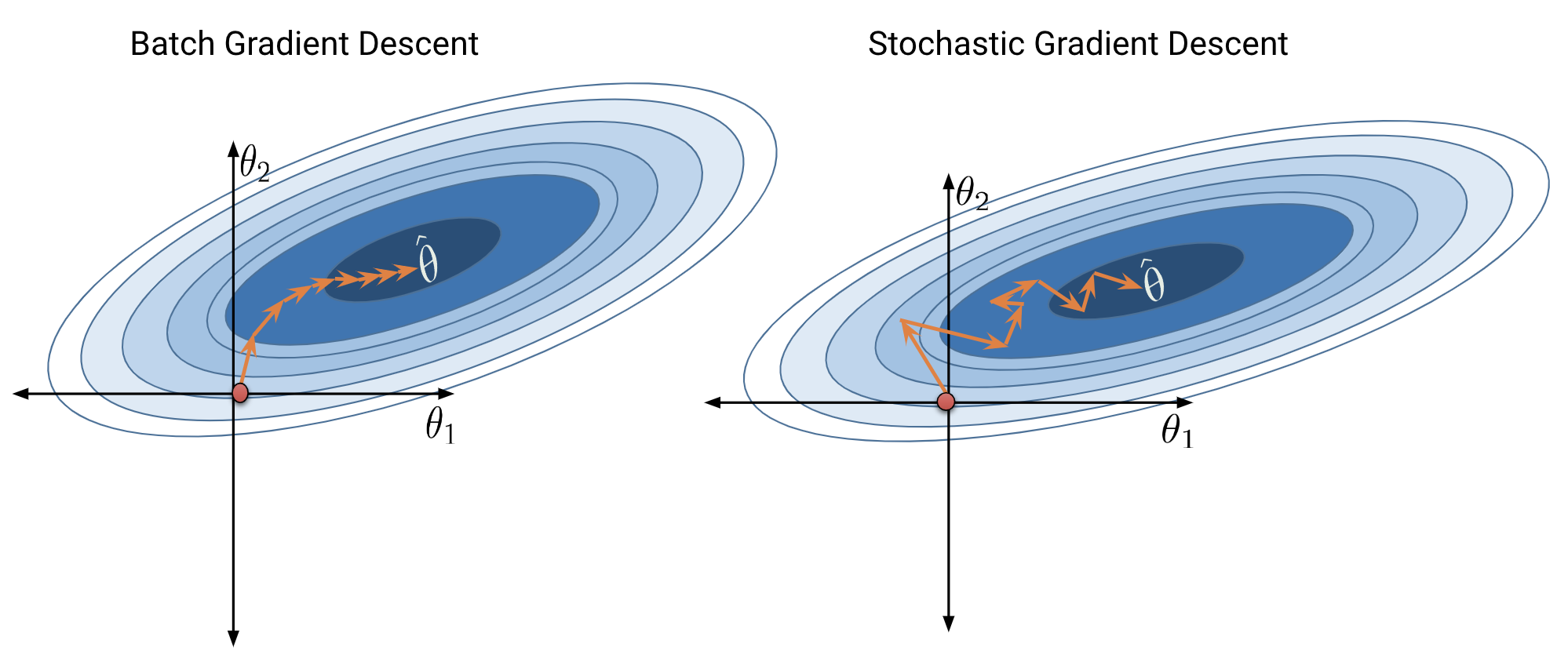
While SGD steps point in the right direction on average, any individual step can be very "noisy." A single data point might be an outlier or simply unusual, and its gradient might point in a direction quite different from the true gradient. This introduces high variance into the optimization process.

Instead of a smooth descent towards the minimum like in BGD, SGD performs a "drunkard's walk." It zig-zags and fluctuates, but the overall trend is towards a region of low loss.

The images below starkly contrast the smooth path of Batch Gradient Descent with the noisy, stochastic path.

The following video contains a fantastic interactive simulation that brings this to life, showing how SGD behaves in practice.

The Practical Standard: Mini-Batch Gradient Descent

We have seen two extremes:

1. Batch Gradient Descent: Uses all $N$ samples. The gradient is accurate (zero variance), but each step is very slow.
2. Stochastic Gradient Descent: Uses 1 sample. Each step is very fast, but the gradient is noisy (high variance).

As is often the case in engineering, the optimal solution lies between these extremes. Mini-Batch Gradient Descent is the de-facto standard in deep learning. It approximates the full gradient by averaging over a small, random subset of the data called a mini-batch of size $B$, where $1<B\ll N$.

The update rule becomes:

where ${\mathcal{B}}_k$ is the set of $B$ indices in the mini-batch at step $k$.

Mini-batching provides two critical advantages:

1. Variance Reduction: By averaging over $B$ samples instead of just one, we get a more accurate estimate of the true gradient. The noise is reduced, leading to more stable convergence than pure SGD.
2. Computational Efficiency: Modern hardware, particularly GPUs, is designed for parallel computation. Processing a single data point (as in pure SGD) does not leverage this parallelism. Processing a mini-batch of, say, 32 or 64 samples allows for highly efficient, vectorized operations that maximize hardware utilization. This is a key insight for anyone interested in high-performance systems.

The following resource clearly defines the terminology and mathematical setup for SGD and mini-batch SGD.

Conclusion

We have successfully derived Stochastic Gradient Descent from first principles, understanding it not as an arbitrary heuristic but as a mathematically-grounded approximation to Batch Gradient Descent. We started with the computational infeasibility of BGD, introduced the idea of using a single sample, and justified it by showing that the stochastic gradient is an unbiased estimator of the true gradient. We then analyzed the trade-off—high variance—and arrived at the practical, efficient middle ground of mini-batch SGD.

Key Takeaways:

• Scalability Problem: BGD is computationally infeasible for large datasets because it requires processing all $N$ data points for every single parameter update.
• Stochastic Approximation: SGD approximates the true gradient using a single, randomly chosen data point. This makes each step $N$ times faster.
• Unbiased but Noisy: The stochastic gradient is an unbiased estimator of the true gradient, ensuring that, on average, SGD moves in the correct direction. However, each individual step is noisy due to high variance.
• Mini-Batch SGD: This is the practical standard. By using a small batch of $B$ samples, it reduces variance compared to pure SGD and leverages hardware parallelism, providing a powerful balance between accuracy and computational speed.

Preview of the Next Lesson:

The noisy nature of SGD, while computationally beneficial, presents its own challenges. The optimizer can get stuck in shallow local minima, struggle on plateaus, or oscillate inefficiently. Our next lesson will introduce Momentum, an elegant technique inspired by physics that helps the optimizer build inertia, smooth out the noisy updates, and accelerate through difficult regions of the loss landscape.