Beyond SGD: Momentum and RMSProp Update Rules

Introduction

In our previous lesson, we established that Stochastic Gradient Descent (SGD) is a computationally efficient and scalable alternative to Batch Gradient Descent. However, we also saw that this efficiency comes at the cost of high variance. The noisy gradient estimates cause the optimization path to oscillate, especially in long, narrow "ravines" of the loss landscape, leading to slow convergence. This erratic behavior can also make it difficult for the optimizer to navigate flat regions or saddle points, where the gradient is close to zero.

This lesson tackles these challenges head-on. We will explore two powerful and widely used enhancements to SGD: Momentum and RMSProp. You will learn how each method incorporates information from past updates to improve the optimization process, but in fundamentally different ways. We will derive their update rules from first principles, understanding how Momentum acts as a "heavy ball" to smooth out oscillations and build speed, while RMSProp adaptively tunes the learning rate for each parameter, allowing for faster progress in complex loss landscapes.

The Problem with SGD: Oscillations and Inefficient Paths

Imagine the contours of a loss function that form a steep, narrow valley. This is a common scenario in neural network optimization. For SGD, the gradient at most points will be large in the direction perpendicular to the valley floor and small in the direction along it.

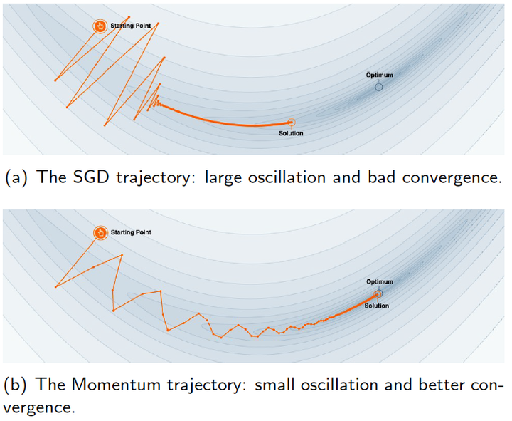
The result is the "zigzag" pattern you see in the image above. The optimizer spends most of its effort oscillating back and forth across the ravine, while making frustratingly slow progress towards the actual minimum at the bottom of the valley.

My question to you: If you were to design a "smarter" update rule, what information from previous steps could you use to mitigate this oscillation? How would you use it to both dampen the unproductive back-and-forth movement and accelerate the productive movement along the valley?

1. Momentum: The Heavy Ball Analogy

Your intuition might lead you to a powerful idea inspired by physics: inertia. A ball rolling down a hill doesn't just stop and change direction instantly. It accumulates momentum, which keeps it moving in a consistent direction and helps it roll over small bumps. We can apply this same principle to our optimizer.

The core idea of Momentum is to not only move in the direction of the current gradient but also to add a fraction of the previous update vector. This creates a "velocity" term that averages out the gradients over time.

This approach is brilliantly explained using a "ball rolling down a hill" analogy in the following video.

The Momentum Update Rule

Let's formalize this. Standard SGD's update is ${\mathbf{w}}_{k+1}={\mathbf{w}}_k-\eta \nabla L({\mathbf{w}}_k)$. The Momentum update introduces a "velocity" vector, $\mathbf{v}$, which is an exponentially weighted moving average of the gradients.

The update proceeds in two steps:

1. Update the velocity vector: $${\mathbf{v}}_k=\beta {\mathbf{v}}_{k-1}+\nabla L({\mathbf{w}}_k)$$
2. Update the weights using the velocity: $${\mathbf{w}}_{k+1}={\mathbf{w}}_k-\eta {\mathbf{v}}_k$$

Here, $\beta$ is the momentum coefficient, typically a value close to 1 (e.g., 0.9). It controls how much of the past velocity is carried over to the current step. When $\beta =0$, we recover standard SGD.

By unrolling the recursion for ${\mathbf{v}}_k$, you can see that it's a weighted sum of all past gradients: ${\mathbf{v}}_k=\nabla L({\mathbf{w}}_k)+\beta \nabla L({\mathbf{w}}_{k-1})+{\beta }^2\nabla L({\mathbf{w}}_{k-2})+\dots$. The gradients from recent steps are given more weight, and the influence of older gradients decays exponentially.

This averaging mechanism is precisely what solves the oscillation problem.

• In directions where gradients consistently point the same way (along the valley), their contributions to the velocity vector add up, accelerating the descent.
• In directions where gradients oscillate (across the valley), their contributions tend to cancel each other out, dampening the unproductive movement.

A Deeper Dive: Accelerated Gradient Descent

The "heavy ball" analogy is intuitive, but the true power of momentum can be understood more formally by analyzing the dynamics of the optimization process. Adding the momentum term effectively transforms the optimization from a first-order system into a second-order one, analogous to a damped harmonic oscillator from classical mechanics. This connection is especially relevant given your engineering background.

A rigorous mathematical treatment by Professor Gilbert Strang shows that with an optimal choice of learning rate $\eta$ and momentum $\beta$, the convergence rate can be dramatically improved. The analysis involves treating the update as a linear dynamical system and finding the parameters that minimize the eigenvalues of the iteration matrix.

This deep dive shows that Momentum is not just a clever heuristic; it is a mathematically grounded method for accelerating convergence.

2. RMSProp: Adapting the Learning Rate

Momentum solves the problem of oscillation. But SGD has another limitation: it uses a single, global learning rate $\eta$ for all parameters. This is often suboptimal. Consider a loss landscape where the curvature varies drastically along different parameter axes.

• Along a very steep, highly curved direction, we need a tiny learning rate to avoid overshooting and diverging.
• Along a very flat direction, we need a large learning rate to make any meaningful progress.

This is where RMSProp (Root Mean Square Propagation) comes in. It's an adaptive learning rate method that maintains a per-parameter learning rate. The key idea is to scale each parameter's update inversely by the magnitude of its recent gradients.

The RMSProp Update Rule

Like Momentum, RMSProp also uses an exponentially weighted moving average, but with a crucial difference. Instead of averaging the gradients themselves, it averages the squared gradients.

1. Maintain a moving average of squared gradients, $S_k$, for each parameter:

   $${\mathbf{S}}_k=\beta {\mathbf{S}}_{k-1}+(1-\beta )(\nabla L({\mathbf{w}}_k){)}^2$$

   Note that the squaring operation $(\cdot {)}^2$ is performed element-wise.

2. Update the weights by dividing the learning rate by the square root of this moving average:

   $${\mathbf{w}}_{k+1}={\mathbf{w}}_k-\frac{\eta }{\sqrt{{\mathbf{S}}_k}+ϵ}\nabla L({\mathbf{w}}_k)$$

Let's break this down:

• ${\mathbf{S}}_k$ tracks the recent average magnitude (squared) of the gradient for each parameter.
• The term $\frac{\eta }{\sqrt{{\mathbf{S}}_k}+ϵ}$ acts as a per-parameter effective learning rate.
• If recent gradients for a parameter have been large, $S_k$ will be large, and the effective learning rate for that parameter will be small. This prevents overshooting in steep directions.
• If recent gradients for a parameter have been small, $S_k$ will be small, and the effective learning rate will be large. This accelerates learning in flat directions.
• $\beta$ is the decay rate, similar to the one in Momentum, typically set to 0.9 or 0.99.
• $ϵ$ is a small constant (e.g., $10^{-8}$) added for numerical stability to prevent division by zero, a detail your systems programming experience will appreciate.

For a clear explanation of this mechanism, let's turn to a textual resource.

Conclusion

In this lesson, we have moved beyond vanilla SGD and derived two advanced optimization techniques that are fundamental to modern deep learning. We saw that while both Momentum and RMSProp use an exponentially weighted moving average to incorporate information from past steps, they do so for entirely different purposes.

Key Takeaways:

• SGD's Challenges: Standard SGD suffers from noisy updates that cause oscillations in narrow ravines and slow progress on flat plateaus. It also uses a single learning rate for all parameters, which is inefficient for complex loss surfaces.
• Momentum:
  • Problem Solved: Dampens oscillations and accelerates convergence.
  • Mechanism: Maintains a moving average of the gradients (the first moment). This builds "velocity" in consistent directions while averaging out oscillating directions.
  • Analogy: A heavy ball rolling downhill, using its inertia to smooth its path.
• RMSProp:
  • Problem Solved: Adapts the learning rate for each parameter individually.
  • Mechanism: Maintains a moving average of the squared gradients (an uncentered second moment). It normalizes the update for each parameter by this magnitude, reducing the step size for large-gradient parameters and increasing it for small-gradient ones.
  • Analogy: A smart hiker who takes small, careful steps on steep terrain and long strides on flat ground.

Preview of the Next Lesson:

We have studied two powerful but distinct ideas. Momentum is about choosing a better direction by accumulating velocity. RMSProp is about choosing a better step size by adapting the learning rate. An obvious and powerful question arises: can we do both? In our next lesson, we will combine these two techniques to derive the Adam (Adaptive Moment Estimation) optimizer, which has become one of the most popular and effective default optimizers for training deep neural networks.