RNN Architecture and the Vanishing Gradient Problem

Introduction

Welcome to the first lesson of our module on sequence modeling! In the previous module, we mastered Convolutional Neural Networks (CNNs), which are experts at processing grid-like data such as images. You learned how to build them, diagnose issues like overfitting, and apply powerful techniques like transfer learning.

Now, we shift our focus to a new and equally important type of data: sequences. This includes time series data (like stock prices), sentences of text, audio signals, and more. Standard neural networks and CNNs are not well-suited for this kind of data because the input length can vary, and the order of the elements is crucial.

In this lesson, we will explore the foundational architecture designed for sequential data: the Recurrent Neural Network (RNN). You will learn:

• The core structure of a simple "vanilla" RNN and how it uses a feedback loop to maintain a "memory" of past information.
• The critical limitation of this simple architecture: the vanishing gradient problem, which prevents it from effectively learning from long sequences.

Understanding this problem is essential, as it motivates the more advanced architectures like LSTMs and GRUs that we will cover next.

1. From Fixed Inputs to Sequences

So far, the networks you've built, like the multi-layer perceptron for binary classification or the CNN for image recognition, have one thing in common: they expect a fixed-size input. A CNN trained on 224x224 pixel images can't directly handle an image of a different size, nor can it process a sequence of images.

But what if our task inherently involves sequences?

• Predicting the next word in a sentence.
• Classifying the sentiment (positive/negative) of a customer review.
• Forecasting tomorrow's weather based on the past week's data.

In these cases, the input isn't a single data point but a sequence of them, and the length of that sequence can change. This is where RNNs come in.

As the video highlights, the key innovation in RNNs is the introduction of feedback loops, which allow the network to process sequential inputs of varying lengths.

2. The Architecture of a Vanilla RNN

The core idea of an RNN is to have a "state" that is updated at each step of a sequence. This state, called the hidden state, acts as the network's memory, capturing information from all previous steps.

An RNN cell takes two inputs at each time step $t$:

1. The current input vector, $x_t$.
2. The hidden state from the previous time step, $h_{t-1}$.

It then produces two outputs:

1. The updated hidden state, $h_t$.
2. An optional output for that time step, $y_t$.

The Recurrence Formula

The process of updating the hidden state is defined by a recurrence formula. For a vanilla RNN, this is typically:

$$h_t=\tanh (W_{hh}{h}_{t-1}+W_{xh}{x}_t+b_h)$$

Let's break this down:

• $h_t$: The new hidden state at time $t$.
• $h_{t-1}$: The hidden state from the previous time step, $t-1$.
• $x_t$: The input at the current time step, $t$.
• $W_{hh}$: A weight matrix that transforms the previous hidden state.
• $W_{xh}$: A weight matrix that transforms the current input.
• $b_h$: A bias term.
• $\tanh$: An activation function that squashes the result into the range [-1, 1], helping to keep the hidden state values bounded.

The output at time step $t$ can then be computed from the hidden state:

$$y_t=W_{hy}{h}_t+b_y$$

A crucial concept here is parameter sharing. The same weight matrices ($W_{hh}$, $W_{xh}$, $W_{hy}$) and biases are used at every single time step. This makes the network incredibly efficient and allows it to generalize to sequences of any length.

To see this process in action, let's visualize how an RNN processes a sequence step-by-step.

3. The Vanishing Gradient Problem

We now have a network that can process sequences. However, vanilla RNNs have a major flaw that makes them difficult to train on long sequences. This is known as the vanishing gradient problem.

Intuition

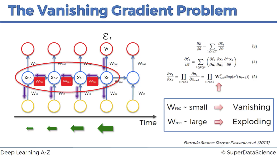
To learn, the network must propagate the error signal from the output back through every time step (a process called Backpropagation Through Time, or BPTT). Imagine a long sentence where the last word depends on the first word. The gradient of the loss with respect to the network's parameters must travel all the way back to the first time step to update the weights correctly.

In a vanilla RNN, this backpropagation process involves repeated matrix multiplications. At each step backward in time, the gradient is multiplied by the recurrent weight matrix $W_{hh}$ and the derivative of the $\tanh$ activation function.

If these factors are, on average, less than 1, the gradient will shrink exponentially as it travels back. After many steps, it becomes so small that it effectively "vanishes," carrying no useful information to update the weights at earlier time steps. The network becomes unable to learn long-range dependencies.

The Mathematical Explanation

Given your background in calculus and linear algebra, we can look at this more formally. The core issue lies in how the gradient of the loss at the final time step $T$, ${\mathcal{L}}_T$, is computed with respect to a hidden state at a much earlier time step $k$. Using the chain rule, this is:

$$\frac{\partial {\mathcal{L}}_T}{\partial h_k}=\frac{\partial {\mathcal{L}}_T}{\partial h_T}\frac{\partial h_T}{\partial h_{T-1}}\frac{\partial h_{T-1}}{\partial h_{T-2}}\cdots \frac{\partial h_{k+1}}{\partial h_k}=\frac{\partial {\mathcal{L}}_T}{\partial h_T}\prod _{t=k+1}^T\frac{\partial h_t}{\partial h_{t-1}}$$

The key term is the product of Jacobians, $\prod \frac{\partial h_t}{\partial h_{t-1}}$. Each Jacobian is:

$$\frac{\partial h_t}{\partial h_{t-1}}=\text{diag}({\tanh }^{\prime }(...))\cdot W_{hh}$$

The derivative of $\tanh$ is always between 0 and 1. This means at every step backward, the gradient is multiplied by a matrix ($W_{hh}$) and then scaled down by the activation derivative. Unless the eigenvalues of $W_{hh}$ are large enough to counteract this, the gradient vector's norm will shrink exponentially.

Exploding Gradients

As mentioned in the article, if the recurrent weights are too large, the opposite can happen: the gradient grows exponentially and "explodes," leading to NaN values and unstable training. This problem, however, is easier to manage. We can use a simple technique called gradient clipping, which just caps the gradient's magnitude at a certain threshold. There is no equally simple fix for a gradient that has vanished to zero.

Let's conclude with a final, intuitive summary of both problems.

Conclusion

In this lesson, you have been introduced to the world of sequence modeling with Recurrent Neural Networks. You now understand the fundamental architecture that allows neural networks to process data where order and context matter.

Key Takeaways:

• RNNs are designed for sequential data of variable length, unlike standard feedforward networks or CNNs.
• They achieve this using a recurrent loop and a hidden state that acts as a memory, carrying information from one time step to the next.
• A key feature of RNNs is parameter sharing: the same set of weights is applied at every step, making them efficient and generalizable.
• The primary weakness of vanilla RNNs is the vanishing gradient problem, where the error signal shrinks exponentially as it propagates back through time.
• This problem arises from the repeated multiplication of matrices during backpropagation and prevents the network from learning long-range dependencies.

The failure of vanilla RNNs to capture long-term context was a major bottleneck in sequence modeling. In our next lesson, we will explore the brilliant architectural solutions designed to overcome this very problem: Long Short-Term Memory (LSTM) and Gated Recurrent Units (GRU). These models introduce "gating" mechanisms that allow the network to control the flow of information, effectively creating a "gradient highway" for learning long-range dependencies.