LSTMs and GRUs: Handling Long-Range Dependencies

Introduction

Welcome back! In our previous lesson, we explored the architecture of a vanilla Recurrent Neural Network (RNN) and identified its critical flaw: the vanishing gradient problem. You learned that due to repeated matrix multiplications during backpropagation, the error signal shrinks exponentially, preventing the network from learning dependencies between distant elements in a sequence. This is why a simple RNN struggles with tasks requiring long-term memory.

In this lesson, we will dissect the ingenious solutions to this problem: Long Short-Term Memory (LSTM) and Gated Recurrent Unit (GRU) networks. These advanced architectures form the backbone of many modern sequence modeling applications. Our goal is to understand precisely how their internal mechanisms, known as "gates," allow them to regulate the flow of information and maintain a memory over long time horizons, effectively solving the long-range dependency problem.

The Core Idea: Selective Memory with Gates

Before diving into the complex diagrams and equations, let's build an intuition for what LSTMs and GRUs do. Think about how you read a long product review. Your brain doesn't store every single word; it learns to identify and remember key phrases like "battery life is terrible" or "screen is amazing," while discarding filler words like "and," "the," or "it." The network needs a similar ability to selectively forget irrelevant information and store important context.

This is precisely what LSTMs and GRUs achieve through gating mechanisms. These gates are small neural networks that learn to control the flow of information, deciding what to keep, what to throw away, and what new information to add to the network's memory.

Long Short-Term Memory (LSTM)

The LSTM, introduced by Hochreiter & Schmidhuber in 1997, was a breakthrough in overcoming the limitations of simple RNNs. Its key innovation is the cell state, which acts as an information highway, allowing context to travel down the sequence with minimal distortion.

The Cell State and Gates

An LSTM cell maintains two vectors that are passed from one time step to the next:

1. Hidden State ($h_t$): This is the same as in a vanilla RNN and serves as the output for the current time step.
2. Cell State ($C_t$): This is the new component. Think of it as the network's long-term memory. The LSTM can read from, write to, and erase information from this cell state.

The flow of information into and out of the cell state is controlled by three gates:

• Forget Gate ($f_t$): Decides what information to discard from the previous cell state ($C_{t-1}$).
• Input Gate ($i_t$): Decides what new information to store in the current cell state ($C_t$).
• Output Gate ($o_t$): Decides which part of the cell state to pass on to the new hidden state ($h_t$).

Each gate is a neural network layer with a sigmoid activation, which outputs values between 0 ("let nothing through") and 1 ("let everything through").

The core operations you just read about can be summarized with these two equations:

1. Cell State Update:

   $$C_t=(f_t\odot C_{t-1})+(i_t\odot {\tilde{C}}_t)$$

   This equation is the heart of the LSTM. We take the old cell state $C_{t-1}$ and multiply it element-wise ($\odot$) by the forget gate's output $f_t$. Then, we add the new candidate information ${\tilde{C}}_t$, scaled by the input gate $i_t$.

2. Hidden State Update:

   $$h_t=o_t\odot \tanh (C_t)$$

   The new hidden state is a filtered version of the new cell state.

How LSTMs Solve Vanishing Gradients

Now we can connect this architecture back to the vanishing gradient problem. In the previous lesson, we saw that the problem arose from the repeated multiplication involving the recurrent weight matrix $W_{hh}$ during backpropagation.

The LSTM's cell state update equation is primarily additive, not multiplicative. This seemingly small change is profound. When we compute the gradient of the loss with respect to the cell state, the chain rule looks very different. The derivative of the current cell state with respect to the previous one, $\frac{\partial C_t}{\partial C_{t-1}}$, is primarily controlled by the forget gate, $f_t$.

By learning to set the forget gate's values, the network can control the gradient flow. If the network needs to remember something for a long time, it can learn to set the corresponding elements of $f_t$ to 1. In this case, the gradient passes through that "memory lane" unchanged, creating a "gradient highway" that doesn't vanish.

This ability to learn when to remember and when to forget is what allows LSTMs to successfully model long-range dependencies where vanilla RNNs fail.

Gated Recurrent Unit (GRU)

The Gated Recurrent Unit (GRU), introduced in 2014, is a popular and effective variation of the LSTM. It aims to achieve the same goal with a simpler architecture.

A GRU cell has two main differences from an LSTM:

1. It combines the cell state and hidden state into a single hidden state vector, $h_t$.
2. It has only two gates instead of three:
   • Update Gate ($z_t$): This gate acts like a combination of the LSTM's forget and input gates. It decides how much of the previous hidden state to keep and what new information to add.
   • Reset Gate ($r_t$): This gate determines how much of the past information to forget when proposing a new candidate hidden state.

This simpler structure makes GRUs computationally more efficient than LSTMs, as they have fewer parameters to train.

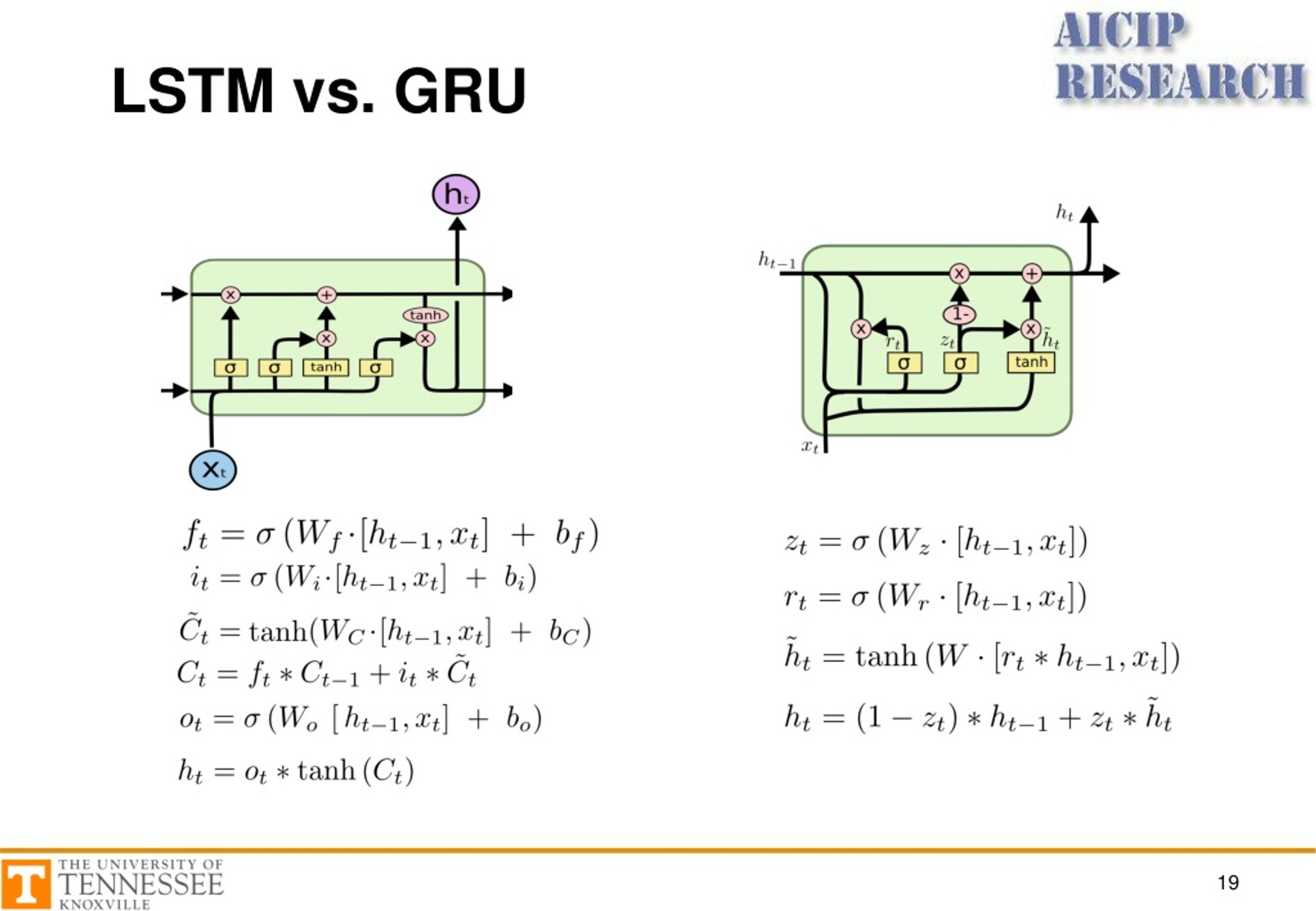
Because GRUs are simpler, they can be faster to train and may require less data to generalize well. However, the LSTM's greater expressive power (with its separate cell state) might give it an edge on very complex tasks with large datasets. In practice, the choice between them is often empirical—you try both and see which one performs better on your specific problem.

Conclusion

In this lesson, you have learned how advanced RNN architectures overcome the vanishing gradient problem that plagues their simpler counterparts.

Key Takeaways:

• LSTMs and GRUs use gating mechanisms to dynamically control the flow of information through the network.
• The LSTM introduces a separate cell state that acts as a "conveyor belt" for information. Its three gates (forget, input, output) learn to protect and control this memory.
• The additive update of the LSTM's cell state is the key to solving the vanishing gradient problem, creating a "gradient highway" that allows the network to learn long-range dependencies.
• The GRU is a simpler and more computationally efficient alternative to the LSTM, using only two gates (update and reset) and a single hidden state vector.
• Both architectures effectively enable networks to learn what to remember and what to forget, making them powerful tools for a wide range of sequence modeling tasks.

Now that you understand the theory behind how these models handle sequences, our next step is to prepare data to feed into them. In the next lesson, we will focus on text preprocessing, specifically a crucial technique called tokenization, which converts raw text into a numerical format that our models can understand.