Kane-Mele Model: Distinguishing Trivial and QSH Insulators

Hello! Welcome back to our exploration of topological matter.

In our last lesson, we introduced the ${\mathbb{Z}}_2$ topological invariant, $\nu$, which classifies insulators that respect time-reversal symmetry. We established that for systems with inversion symmetry, this invariant can be calculated with surprising ease using the Fu-Kane formula, which relates $\nu$ to the parity eigenvalues of the occupied bands at the time-reversal invariant momenta (TRIMs):

A result of $-1$ signals a topological insulator ($\nu =1$), while $+1$ indicates a trivial one ($\nu =0$).

Today, we will bring this abstract concept to life by analyzing the quintessential model of a 2D topological insulator: the Kane-Mele model. Our goal is to use this model to understand the physical difference between a trivial insulator and a Quantum Spin Hall (QSH) insulator, which is the physical realization of a 2D, ${\mathbb{Z}}_2$ topological insulator. We will see how a specific physical interaction—spin-orbit coupling—can drive a system from a trivial to a topological phase, and how this is reflected in both the bulk topological invariant and the appearance of characteristic edge states.

1. From Graphene to the Quantum Spin Hall Effect

The story of the Kane-Mele model begins with graphene. As you know from your study of band theory, graphene's unique honeycomb lattice gives rise to a semimetallic band structure with gapless Dirac cones at the $K$ and $K^{\prime }$ points of the Brillouin zone. To create an insulator, we must open a gap at these points. There are two primary ways to do this:

1. Break Sublattice Symmetry: Apply a staggered potential, $m$, that gives different on-site energies to the A and B sublattices. This breaks inversion symmetry and opens a gap, but as we will see, it leads to a topologically trivial insulator.
2. Introduce Intrinsic Spin-Orbit Coupling (SOC): Add a term that couples an electron's spin to its motion. The crucial insight of Kane and Mele was to consider a specific, time-reversal symmetric form of SOC. This also opens a gap, but it results in a fundamentally different state: the Quantum Spin Hall (QSH) insulator.

To get a feel for the core idea, let's hear from one of its originators, Charles Kane.

This idea of "two copies of the quantum Hall effect" is central. The intrinsic SOC in the Kane-Mele model acts like an effective magnetic field that points up for spin-up electrons and down for spin-down electrons. This generates a spin-up Hall current in one direction and a spin-down Hall current in the other. The net charge current is zero, but there is a net flow of spin—a spin current. This is the essence of the Quantum Spin Hall effect.

2. The Kane-Mele Hamiltonian and Topological Invariant

To make this precise, we need to analyze the model's Hamiltonian. While the full tight-binding model is important for numerical work, a simplified 4x4 effective Hamiltonian captures the low-energy physics around the Dirac points and is ideal for our analysis.

Let's summarize and connect the key points from the reading to what we learned in the previous lesson.

The effective Hamiltonian can be written as:

In this simplified model:

• The basis is $(A\uparrow ,A\downarrow ,B\uparrow ,B\downarrow )$.
• ${\Gamma }_1={\sigma }_x\otimes I$ and ${\Gamma }_2={\sigma }_y\otimes I$ represent the nearest-neighbor hopping of graphene, where ${\sigma }_i$ act on the sublattice space.
• ${\Gamma }_3={\sigma }_z\otimes s_z$ represents the intrinsic SOC term.
• The model also has inversion symmetry, represented by the parity operator $P={\sigma }_x\otimes I={\Gamma }_1$.

The crucial step is to apply the Fu-Kane formula from our previous lesson. We need the parity eigenvalues of the occupied bands at the TRIMs. The reading shows that at a TRIM ${\mathbf{\Lambda }}_i$, the functions $d_2$ and $d_3$ vanish due to symmetry, so $H({\mathbf{\Lambda }}_i)=d_1({\mathbf{\Lambda }}_i){\Gamma }_1$.

The eigenstates of this Hamiltonian are also eigenstates of the parity operator ${\Gamma }_1$, with eigenvalues $\zeta =\pm 1$. The corresponding energy eigenvalues are $E=\pm d_1({\mathbf{\Lambda }}_i)$. The occupied (valence) band will have negative energy. Its parity eigenvalue ${\zeta }_{-}({\mathbf{\Lambda }}_i)$ will therefore depend on the sign of $d_1({\mathbf{\Lambda }}_i)$. A careful check shows ${\zeta }_{-}({\mathbf{\Lambda }}_i)\propto \text{sign}(d_1({\mathbf{\Lambda }}_i))$.

Plugging this into the Fu-Kane formula for the two occupied bands (which form a Kramers pair):

Since the number of TRIMs in 2D is even (four), the proportionality constant drops out, and we arrive at the elegant result from the paper (Eq. 46):

Here, the function $d_1(\mathbf{k})$ incorporates both the graphene hopping terms and any sublattice-symmetry-breaking staggered potential $m$. A typical form is $d_1(\mathbf{k})\approx m-{\lambda }_{SO}f(\mathbf{k})$, where ${\lambda }_{SO}$ is the SOC strength and $f(\mathbf{k})$ is some function.

This gives us a clear distinction:

• Trivial Insulator ($\nu =0$): $\prod \text{sign }{d}_1({\mathbf{\Lambda }}_i)=+1$. This happens if $d_1$ has the same sign at all TRIMs (e.g., when a large staggered potential $m$ dominates) or changes sign at an even number of TRIMs.
• Topological Insulator ($\nu =1$): $\prod \text{sign }{d}_1({\mathbf{\Lambda }}_i)=-1$. This occurs if $d_1$ changes sign at an odd number of TRIMs. This is the signature of a band inversion, where the SOC term becomes strong enough to invert the natural order of the bands at one of the TRIMs.

3. Seeing the Difference: Bulk-Boundary Correspondence

The bulk topological invariant $\nu$ has a dramatic consequence at the system's boundary. The bulk-boundary correspondence principle for ${\mathbb{Z}}_2$ insulators states that a system with $\nu =1$ must host gapless states at its edge that are protected by time-reversal symmetry. A trivial insulator ($\nu =0$) has no such guarantee.

Given your background in computational physics, the most direct way to observe this is to implement and solve the model numerically.

Mini-Project: Numerical Analysis of the Kane-Mele Model

Let's put theory into practice. Your task is to numerically diagonalize the Kane-Mele model on a honeycomb lattice configured as a finite strip (often called a "zigzag nanoribbon"). This setup is periodic in one direction (say, $y$) and has open boundaries in the other ($x$). This allows us to plot the band structure $E$ as a function of the conserved momentum $k_y$ and see if any states appear at the edges.

The resource LINK provides a detailed problem set that walks through this exact task.

Your Goal:
Using your preferred programming language (Python, Julia, Matlab), implement the tight-binding Hamiltonian for the Kane-Mele model on a strip and plot its energy spectrum $E(k_y)$. You should reproduce the key distinction between a trivial and a topological insulator.

Steps:

1. Set up the Hamiltonian: Use "Problem 3: Edge modes of the Kane-Mele model" from LINK as your guide. It provides the full real-space Hamiltonian (Eq. 16) and derives the block-tridiagonal matrix form $H(k_y)$ for a strip geometry (Eqs. 18-21).
2. Case 1: Trivial Insulator. Set the SOC to zero (${\lambda }_{SO}=0$) and introduce a small staggered potential ($m\approx 0.2$). Diagonalize $H(k_y)$ for a range of $k_y$ in the Brillouin zone and plot the eigenvalues. You should observe that a gap opens across the entire spectrum. The system is fully insulating.
3. Case 2: QSH Insulator. Now, switch off the staggered potential ($m=0$) and turn on a small amount of SOC (${\lambda }_{SO}\approx 0.05$). Re-run your diagonalization. You will see a gap open in the "bulk" bands, but crucially, you will also see new states that traverse the bulk gap. These are the topologically protected helical edge states.

Your plot for the QSH phase should resemble the one below, which shows a gapped bulk spectrum with states crossing the gap.

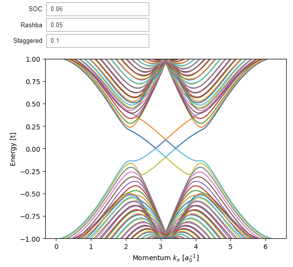
4. (Optional but Recommended) The Phase Transition: As described in part (e) of the problem set, start from the QSH phase (finite ${\lambda }_{SO}$, zero $m$) and gradually increase the staggered potential $m$. You will see the bulk gap close at a critical value of $m$ and then reopen. Past this critical point, the edge states will disappear. You have driven the system through a topological phase transition into a trivial insulator! This transition corresponds exactly to the point where the product of signs of $d_1$ at the TRIMs flips from $-1$ to $+1$.

This numerical exercise provides a powerful visual confirmation of the bulk-boundary correspondence. The abstract bulk invariant $\nu =1$, calculated from parity eigenvalues, manifests as concrete, physically observable conducting channels at the edge of the material.

Conclusion

Today we dissected the Kane-Mele model, our first concrete example of a time-reversal invariant topological insulator. We have seen how the interplay between different gap-opening mechanisms—a trivial staggered potential versus a topological spin-orbit coupling—leads to two distinct insulating phases.

Key Takeaways:

• The Kane-Mele model describes graphene with an intrinsic, time-reversal symmetric spin-orbit coupling.
• This SOC term can drive a band inversion at an odd number of TRIMs, changing the ${\mathbb{Z}}_2$ invariant from $\nu =0$ (trivial) to $\nu =1$ (topological).
• The distinction between the trivial and topological (QSH) phases is determined by the sign of a term in the Hamiltonian at the four TRIMs, which connects directly to the Fu-Kane parity formula.
• The hallmark of the QSH phase ($\nu =1$) is the guaranteed existence of gapless edge states, which can be clearly visualized by solving the model on a strip geometry. A trivial insulator ($\nu =0$) does not have such protected states.

Preview of the Next Lesson

We've now seen that the edge states exist. But what are their properties? In the next lesson, we will zoom in on these helical edge states. We will analyze their wavefunctions to understand their most defining characteristic: spin-momentum locking. This property, where spin-up electrons propagate in one direction along the edge and spin-down in the other, is the reason for their remarkable robustness and is the key to many of the proposed applications of topological insulators.