Measuring Entanglement: Purity and Von Neumann Entropy

Hello! Welcome to the next lesson in our module on Open Quantum Systems and Measurement.

In our last session, we mastered the partial trace, a crucial tool for isolating and describing a subsystem $\text{A}$ when it's part of a larger quantum system $\text{A+B}$. We made a critical observation: even if the total system $\text{A+B}$ is in a pure state, its subsystem $\text{A}$ is generally in a mixed state if the two are entangled. The "mixedness" of the subsystem's reduced density matrix, ${\hat{\rho }}_A$, is a direct fingerprint of this entanglement.

Today, we will build directly on that foundation to achieve our learning outcome: to quantify entanglement using purity and von Neumann entropy. We'll move beyond a simple yes/no answer to "is it entangled?" and learn how to answer "by how much?". These measures are not just abstract concepts; they are essential tools in modern condensed matter physics for characterizing quantum phases of matter, understanding thermalization in isolated systems, and quantifying resources in quantum computation.

1. Purity: A First Look at Entanglement

We've already encountered the purity, $\gamma =\text{Tr}({\hat{\rho }}^2)$, as a simple test for whether a state is pure or mixed. Let's formalize its role as a measure of entanglement. When we have a bipartite system $\text{A+B}$ in a pure state, the purity of the reduced density matrix ${\hat{\rho }}_A$ tells us about the entanglement between $\text{A}$ and $\text{B}$.

• If $\text{A}$ and $\text{B}$ are not entangled (i.e., the total state is a product state), then ${\hat{\rho }}_A$ is pure, and its purity is $\gamma ({\hat{\rho }}_A)=1$.
• If $\text{A}$ and $\text{B}$ are entangled, ${\hat{\rho }}_A$ is mixed, and its purity is $\gamma ({\hat{\rho }}_A)<1$. The more entangled the state, the more mixed ${\hat{\rho }}_A$ becomes, and the lower its purity.
• For a subsystem with a $d$-dimensional Hilbert space, the minimum possible purity is $1/d$, corresponding to a maximally mixed state, which arises from maximal entanglement with another system.

Purity is useful for a quick check, but it lacks some of the deeper properties and interpretations of a true information-theoretic measure. For that, we need to introduce a more powerful concept.

2. The Von Neumann Entropy

The proper quantum mechanical analogue of classical Shannon entropy is the von Neumann entropy. For a system described by a density matrix $\hat{\rho }$, it is defined as:

$$S(\hat{\rho })=-\text{Tr}(\hat{\rho }\ln \hat{\rho })$$

This definition might seem abstract, but it becomes much clearer when we consider the eigenvalues of the density matrix. Since $\hat{\rho }$ is Hermitian, it can be diagonalized. Let its eigenvalues be $\{{\lambda }_i\}$. In the basis where $\hat{\rho }$ is diagonal, the operator $\ln \hat{\rho }$ is also diagonal with elements $\ln {\lambda }_i$. The calculation of the trace then simplifies dramatically:

$$S(\hat{\rho })=-\sum _i{\lambda }_i\ln {\lambda }_i$$

This looks exactly like the Shannon entropy for a classical probability distribution given by the eigenvalues $\{{\lambda }_i\}$.

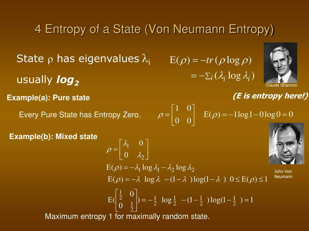
The von Neumann entropy has several key properties that make it a robust measure of the "mixedness" or uncertainty in a quantum state:

1. Non-negativity: $S(\hat{\rho })\ge 0$.
2. Pure States: $S(\hat{\rho })=0$ if and only if $\hat{\rho }$ is a pure state. In this case, one eigenvalue is 1 and all others are 0, so $S=-(1\ln 1)=0$. There is no uncertainty.
3. Maximally Mixed States: The entropy is maximum for a maximally mixed state, where $\hat{\rho }=\frac{1}{d}\hat{I}$. In this case, all $d$ eigenvalues are $1/d$, and the entropy is $S(\hat{\rho })=-{\sum }_{i=1}^d\frac{1}{d}\ln (\frac{1}{d})=\ln d$. There is maximum uncertainty.

To see a clear, pedagogical breakdown of these properties, please watch the following video.

3. Entanglement Entropy: Quantifying Quantum Connection

Now we can combine the concepts from the last two lessons. We have a way to describe a subsystem (${\hat{\rho }}_A={\text{Tr}}_B({\hat{\rho }}_{AB})$) and a way to quantify its mixedness ($S({\hat{\rho }}_A)$). This leads us to the central definition of this lesson.

For a bipartite system $\text{A+B}$ in a pure state $|\Psi {⟩}_{AB}$, the entanglement entropy is defined as the von Neumann entropy of the reduced density matrix of either subsystem.

$$S_E=S({\hat{\rho }}_A)=-{\text{Tr}}_A({\hat{\rho }}_A\ln {\hat{\rho }}_A)$$

Crucially, it can be proven that for a pure state of the composite system, the entropy of both subsystems is identical: $S({\hat{\rho }}_A)=S({\hat{\rho }}_B)$. Entanglement is a shared property.

The entanglement entropy $S_E$ directly quantifies the amount of entanglement between $\text{A}$ and $\text{B}$.

• If $S_E=0$, the subsystems are not entangled.
• If $S_E>0$, the subsystems are entangled. The larger the value, the greater the entanglement.

This concept is so fundamental that it bridges quantum mechanics with statistical mechanics and information theory. The following reading from Leo Radzihovsky's lecture notes formalizes this idea and provides clear examples.

The key insight is that the entropy of a subsystem doesn't come from classical ignorance about its state, but from purely quantum correlations with another system. All the information is encoded in the non-local correlations, making the local state appear random.

4. Calculating Entanglement Entropy

Let's make this concrete. Consider the state we analyzed in the previous lesson's exercise:

$$|\Psi {⟩}_{AB}=\alpha |0_A{0}_B⟩+\beta |1_A{1}_B⟩(\text{with }{\alpha }^2+{\beta }^2=1)$$

We found the reduced density matrix for subsystem A to be:

$${\hat{\rho }}_A=\left(\begin{array}{cc}{\alpha }^2& 0\\ 0& {\beta }^2\end{array}\right)$$

The eigenvalues are simply ${\lambda }_1={\alpha }^2$ and ${\lambda }_2={\beta }^2$. The entanglement entropy is therefore:

$$S_E=S({\hat{\rho }}_A)=-({\alpha }^2\ln {\alpha }^2+{\beta }^2\ln {\beta }^2)$$

Let's check the limits:

• Product state (e.g., $\alpha =1,\beta =0$): $S_E=-(1\ln 1+0\ln 0)=0$. No entanglement.
• Maximally entangled Bell state ($\alpha =\beta =1/\sqrt{2}$): $S_E=-(\frac{1}{2}\ln \frac{1}{2}+\frac{1}{2}\ln \frac{1}{2})=-\ln \frac{1}{2}=\ln 2$. This is the maximum entropy for a single qubit and corresponds to one "ebit" (entangled bit) of entanglement.

The Schmidt Decomposition

Calculating eigenvalues for large matrices can be difficult. Fortunately, for bipartite pure states, there is a powerful mathematical tool called the Schmidt decomposition. It states that any pure state $|\Psi {⟩}_{AB}$ can be written in the special form:

$$|\Psi {⟩}_{AB}=\sum _{k=1}^r{\lambda }_k|u_k{⟩}_A|v_k{⟩}_B$$

where $\{|u_k{⟩}_A\}$ and $\{|v_k{⟩}_B\}$ are orthonormal sets of states for their respective subsystems, and the ${\lambda }_k$ are non-negative real numbers called Schmidt coefficients, satisfying ${\sum }_k{\lambda }_k^2=1$. The number of non-zero coefficients, $r$, is the Schmidt rank.

The magic of this decomposition is that the squared Schmidt coefficients, ${\lambda }_k^2$, are precisely the non-zero eigenvalues of the reduced density matrices ${\hat{\rho }}_A$ and ${\hat{\rho }}_B$. This gives us a direct way to compute the entanglement entropy:

$$S_E=-\sum _{k=1}^r{\lambda }_k^2\ln ({\lambda }_k^2)$$

A state is entangled if and only if its Schmidt rank $r>1$.

The following notes provide a clear explanation of Schmidt decomposition and its connection to entanglement entropy.

Test your understanding!

Consider the following two-qubit state:

$$|\varphi ⟩=\frac{1}{\sqrt{3}}|00⟩+\sqrt{\frac{2}{3}}|11⟩$$

This state is already in Schmidt form.

1. What are the Schmidt coefficients?
2. What are the eigenvalues of the reduced density matrix ${\hat{\rho }}_A$?
3. Calculate the purity $\gamma ({\hat{\rho }}_A)$.
4. Calculate the entanglement entropy $S_E$. Is the state more or less entangled than a Bell state?

Show answer

1. The Schmidt coefficients are ${\lambda }_0=1/\sqrt{3}$ and ${\lambda }_1=\sqrt{2/3}$.

2. The eigenvalues of ${\hat{\rho }}_A$ are the squares of the Schmidt coefficients: ${\lambda }_0^2=1/3$ and ${\lambda }_1^2=2/3$. The reduced density matrix is ${\hat{\rho }}_A=\text{diag}(1/3,2/3)$.

3. The purity is $\gamma ({\hat{\rho }}_A)=\text{Tr}({\hat{\rho }}_A^2)=(1/3{)}^2+(2/3{)}^2=1/9+4/9=5/9$.
   Since $\gamma <1$, the state is entangled. For a Bell state, the purity would be $1/2$. Since $5/9>1/2$, we can guess that this state is less entangled.

4. The entanglement entropy is:

   $$S_E=-\left(\frac{1}{3}\ln \frac{1}{3}+\frac{2}{3}\ln \frac{2}{3}\right)=-\left(-\frac{\ln 3}{3}+\frac{2}{3}(\ln 2-\ln 3)\right)=\frac{\ln 3}{3}-\frac{2\ln 2}{3}+\frac{2\ln 3}{3}=\ln 3-\frac{2}{3}\ln 2$$

   Numerically, $S_E\approx 1.0986-\frac{2}{3}(0.6931)\approx 0.6365$.
   For a Bell state, the entropy is $\ln 2\approx 0.6931$. Since $0.6365<0.6931$, this state is indeed less entangled than a maximally entangled Bell state.

Conclusion

In this lesson, we have developed the primary tools for quantifying quantum entanglement in bipartite systems.

Key Takeaways:

• For a pure bipartite state, the "mixedness" of a subsystem's reduced density matrix is a direct measure of its entanglement with the other part.
• Purity, $\gamma =\text{Tr}({\hat{\rho }}^2)$, is a simple indicator of mixedness, where $\gamma =1$ means pure (no entanglement) and $\gamma <1$ means mixed (entangled).
• Von Neumann Entropy, $S(\hat{\rho })=-\text{Tr}(\hat{\rho }\ln \hat{\rho })$, is the definitive measure of mixedness and uncertainty in a quantum state.
• Entanglement Entropy, $S_E$, is the von Neumann entropy of a subsystem's reduced density matrix. For a pure bipartite state, it quantifies the entanglement, ranging from 0 for a product state to $\ln d$ for a maximally entangled state in $d\times d$ dimensions.
• The Schmidt decomposition is a powerful technique that simplifies the calculation of entanglement entropy by directly providing the eigenvalues of the reduced density matrices.

Preview of the Next Lesson:
So far, we have focused on a static picture: describing a subsystem and quantifying its entanglement at a single point in time. In the next lesson, we will turn to dynamics. We will begin to model how an open quantum system evolves under the influence of its environment, leading to phenomena like decoherence and dissipation, using the powerful Lindblad master equation.