Partial Trace and Reduced Density Matrices

Hello! Welcome back to our module on Open Quantum Systems and Measurement.

In our last lesson, we established the density matrix, $\hat{\rho }$, as a powerful tool for describing quantum systems, whether they are in a pure state of perfect knowledge or a mixed state of statistical uncertainty. We saw that for any closed system, its dynamics are governed by the von Neumann equation.

However, in the real world, and especially in condensed matter systems, perfect isolation is an idealization. More often, the system we care about (let's call it A) is just one part of a larger composite system (A+B), where B might be another particle, a set of nuclear spins, or an entire thermal reservoir. If system A is entangled with B, we can no longer describe A with its own independent state vector. This is where the density matrix formalism truly shines.

Today, we will learn how to obtain a complete description of subsystem A, even when it's entangled with B. Our learning outcome is to calculate partial traces to obtain reduced density matrices for subsystems. This procedure of "tracing out" the environment is a cornerstone of modern quantum physics and is the essential prerequisite for quantifying entanglement, which we will tackle in our next lesson.

1. Describing a Subsystem: The Reduced Density Matrix

Imagine a composite system with Hilbert space $\mathcal{H}={\mathcal{H}}_A\otimes {\mathcal{H}}_B$. The full system is described by a density matrix ${\hat{\rho }}_{AB}$. Now, suppose we want to measure an observable ${\hat{O}}_A$ that acts only on subsystem A. In the full Hilbert space, this observable is represented by the operator ${\hat{O}}_A\otimes {\hat{I}}_B$, where ${\hat{I}}_B$ is the identity on ${\mathcal{H}}_B$.

The expectation value is given by the rule we learned:

$$⟨{\hat{O}}_A⟩={\text{Tr}}_{AB}({\hat{\rho }}_{AB}({\hat{O}}_A\otimes {\hat{I}}_B))$$

The trace is taken over the entire Hilbert space ${\mathcal{H}}_{AB}$. This is cumbersome if we only care about subsystem A. Our goal is to find an operator ${\hat{\rho }}_A$ that lives only in ${\mathcal{H}}_A$ and satisfies the simpler relation:

$$⟨{\hat{O}}_A⟩={\text{Tr}}_A({\hat{\rho }}_A{\hat{O}}_A)$$

This operator, ${\hat{\rho }}_A$, is called the reduced density matrix of subsystem A. It is obtained from the full density matrix by performing a partial trace over subsystem B, denoted as ${\hat{\rho }}_A={\text{Tr}}_B({\hat{\rho }}_{AB})$.

2. The Partial Trace Operation

The partial trace over B is formally defined as follows. Let $\{|v_k{⟩}_B\}$ be any orthonormal basis for subsystem B's Hilbert space, ${\mathcal{H}}_B$. Then the partial trace is:

$${\hat{\rho }}_A={\text{Tr}}_B({\hat{\rho }}_{AB})=\sum _k⟨v_k{|}_B{\hat{\rho }}_{AB}|v_k{⟩}_B$$

In words, we are "sandwiching" the full density matrix between the basis states of the subsystem we want to ignore (B) and then summing over all those basis states. The result is an operator that acts solely on the remaining space (A).

To understand the definition and build intuition for why it works, the following video provides an excellent formal introduction. It starts by showing how the partial trace correctly reduces to the subsystem's density matrix for a simple, non-entangled (separable) state.

The key insight is that by summing over a complete basis for B, we are effectively averaging over all possible outcomes for B, leaving us with a description that is valid irrespective of the state of B.

3. Calculating the Reduced Density Matrix: A Concrete Example

The true power of the partial trace becomes evident when dealing with entangled states. Let's take the canonical example of two qubits, A ("Alice") and B ("Bob"), prepared in a Bell state:

$$|\Psi {⟩}_{AB}=\frac{1}{\sqrt{2}}(|0{⟩}_A|0{⟩}_B+|1{⟩}_A|1{⟩}_B)$$

The system as a whole is in a pure state. The full density matrix is ${\hat{\rho }}_{AB}=|\Psi {⟩}_{AB}⟨\Psi {|}_{AB}$:

$${\hat{\rho }}_{AB}=\frac{1}{2}\left(|00⟩⟨00|+|00⟩⟨11|+|11⟩⟨00|+|11⟩⟨11|\right)$$

Let's find Bob's reduced density matrix, ${\hat{\rho }}_B={\text{Tr}}_A({\hat{\rho }}_{AB})$. We need to trace over Alice's basis states, $\{|0{⟩}_A,|1{⟩}_A\}$.

$${\hat{\rho }}_B=⟨0{|}_A{\hat{\rho }}_{AB}|0{⟩}_A+⟨1{|}_A{\hat{\rho }}_{AB}|1{⟩}_A$$

This calculation requires careful application of inner products in the tensor product space. The following video provides a very clear, step-by-step walkthrough of this exact calculation.

After the calculation, we arrive at a remarkable result for Bob's state:

$${\hat{\rho }}_B=\frac{1}{2}|0{⟩}_B⟨0{|}_B+\frac{1}{2}|1{⟩}_B⟨1{|}_B=\frac{1}{2}\left(\begin{array}{cc}1& 0\\ 0& 1\end{array}\right)=\frac{1}{2}{\hat{I}}_B$$

This is a maximally mixed state. Even though the composite system A+B was in a perfectly defined pure state, the state of the subsystem B is completely random. This is a profound consequence of entanglement. All information is stored in the correlations between A and B, not in the individual subsystems.

We can verify this using the purity test from our last lesson:

$$\text{Tr}({\hat{\rho }}_B^2)=\text{Tr}\left(\frac{1}{4}{\hat{I}}_B\right)=\frac{1}{4}\text{Tr}({\hat{I}}_B)=\frac{1}{4}(1+1)=\frac{1}{2}<1$$

Since the purity is less than 1, the state is indeed mixed.

4. The Partial Trace in Matrix Form

Given your computational background, it's useful to see how the partial trace works at the level of matrices. If you write the full density matrix ${\rho }_{AB}$ as a block matrix, where each block corresponds to an element of A's density matrix, the partial trace over B is simply the sum of the diagonal blocks.

Let's use the basis $|00⟩,|01⟩,|10⟩,|11⟩$. The Bell state density matrix is:

$${\rho }_{AB}=\frac{1}{2}\left(\begin{array}{cccc}1& 0& 0& 1\\ 0& 0& 0& 0\\ 0& 0& 0& 0\\ 1& 0& 0& 1\end{array}\right)$$

To get ${\rho }_A={\text{Tr}}_B({\rho }_{AB})$, we can view this as a 2x2 block matrix, where each block is a 2x2 matrix in B's space:

$${\rho }_{AB}=\left(\begin{array}{cc}{M}_{00}& M_{01}\\ M_{10}& M_{11}\end{array}\right)\text{where}({\rho }_A{)}_{ij}=\text{Tr}(M_{ij})$$

In our case:

$$M_{00}=\frac{1}{2}\left(\begin{array}{cc}1& 0\\ 0& 0\end{array}\right),M_{01}=\frac{1}{2}\left(\begin{array}{cc}0& 1\\ 0& 0\end{array}\right)$$ $$M_{10}=\frac{1}{2}\left(\begin{array}{cc}0& 0\\ 1& 0\end{array}\right),M_{11}=\frac{1}{2}\left(\begin{array}{cc}0& 0\\ 0& 1\end{array}\right)$$

Then the elements of ${\rho }_A$ are:

$$({\rho }_A{)}_{00}=\text{Tr}(M_{00})=\frac{1}{2},({\rho }_A{)}_{01}=\text{Tr}(M_{01})=0$$ $$({\rho }_A{)}_{10}=\text{Tr}(M_{10})=0,({\rho }_A{)}_{11}=\text{Tr}(M_{11})=\frac{1}{2}$$

This gives ${\rho }_A=\frac{1}{2}\left(\begin{array}{cc}1& 0\\ 0& 1\end{array}\right)$, the same result as for ${\rho }_B$.

The following image provides a helpful visual for this process.

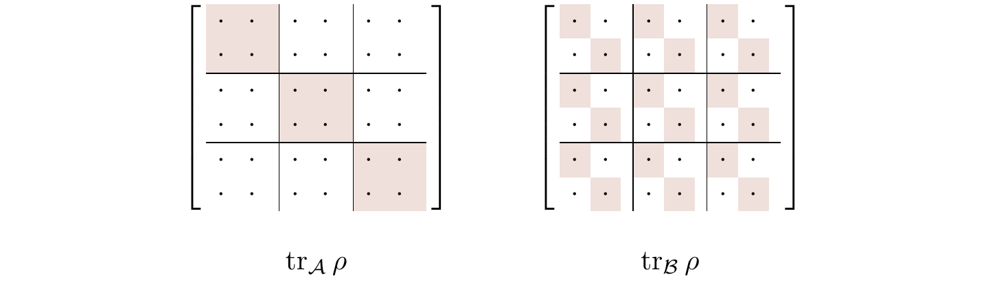
This matrix perspective is extremely useful for implementing calculations numerically, for instance in Python with NumPy, where you can manipulate blocks of matrices directly.

Test your understanding!

Consider a non-maximally entangled state of two qubits:

$$|\Psi ⟩=\alpha |0_A{0}_B⟩+\beta |1_A{1}_B⟩$$

where $\alpha ,\beta$ are real coefficients satisfying ${\alpha }^2+{\beta }^2=1$.

1. Calculate the reduced density matrix for subsystem A, ${\hat{\rho }}_A$.
2. Calculate the purity of ${\hat{\rho }}_A$. For what values of $\alpha$ and $\beta$ is the subsystem in a pure state? When is it maximally mixed?

Show answer

1. First, we write the full density matrix ${\hat{\rho }}_{AB}=|\Psi ⟩⟨\Psi |$:

   $${\hat{\rho }}_{AB}=(\alpha |00⟩+\beta |11⟩)(\alpha ⟨00|+\beta ⟨11|)={\alpha }^2|00⟩⟨00|+\alpha \beta |00⟩⟨11|+\alpha \beta |11⟩⟨00|+{\beta }^2|11⟩⟨11|$$

   Now, we trace over subsystem B's basis $\{|0_B⟩,|1_B⟩\}$:

   $${\hat{\rho }}_A={\text{Tr}}_B({\hat{\rho }}_{AB})=⟨0_B|{\hat{\rho }}_{AB}|0_B⟩+⟨1_B|{\hat{\rho }}_{AB}|1_B⟩$$

   Let's evaluate the terms. Using $⟨i_B|j_B{k}_B⟩={\delta }_{ij}|k_B⟩$ and $⟨j_B{k}_B|i_B⟩={\delta }_{ik}⟨j_B|$:
   \begin{align*}
   \langle0_B|\hat{\rho}{AB}|0_B\rangle &= \alpha^2 |0_A\rangle\langle0_A| \langle0_B|0_B\rangle\langle0_B|0_B\rangle = \alpha^2 |0_A\rangle\langle0_A| \
   \langle1_B|\hat{\rho}{AB}|1_B\rangle &= \beta^2 |1_A\rangle\langle1_A| \langle1_B|1_B\rangle\langle1_B|1_B\rangle = \beta^2 |1_A\rangle\langle1_A|
   \end{align*}
   All cross-terms like $⟨0_B|00⟩⟨11|0_B⟩$ are zero because of orthogonality. So, the reduced density matrix is:

   $${\hat{\rho }}_A={\alpha }^2|0_A⟩⟨0_A|+{\beta }^2|1_A⟩⟨1_A|=\left(\begin{array}{cc}{\alpha }^2& 0\\ 0& {\beta }^2\end{array}\right)$$

2. To find the purity, we calculate $\gamma =\text{Tr}({\hat{\rho }}_A^2)$:

   $${\hat{\rho }}_A^2=\left(\begin{array}{cc}{\alpha }^2& 0\\ 0& {\beta }^2\end{array}\right)\left(\begin{array}{cc}{\alpha }^2& 0\\ 0& {\beta }^2\end{array}\right)=\left(\begin{array}{cc}{\alpha }^4& 0\\ 0& {\beta }^4\end{array}\right)$$ $$\gamma =\text{Tr}({\hat{\rho }}_A^2)={\alpha }^4+{\beta }^4$$

   The subsystem A is in a pure state if $\gamma =1$. Given ${\alpha }^2+{\beta }^2=1$, ${\alpha }^4+{\beta }^4=1$ only if $\alpha =0,\beta =1$ or $\alpha =1,\beta =0$. This corresponds to the unentangled product states $|11⟩$ and $|00⟩$, which makes perfect sense.
   The state is maximally mixed when the purity is at its minimum. This occurs when $\alpha =\beta =1/\sqrt{2}$, which gives $\gamma =(1/2{)}^2+(1/2{)}^2=1/2$. This corresponds to the Bell state we analyzed earlier.

Conclusion

Today we have introduced a fundamental operation in quantum mechanics: the partial trace. It is the mathematical tool that lets us "zoom in" on a part of a larger quantum system, providing a complete statistical description of that subsystem via its reduced density matrix.

Key Takeaways:

• The reduced density matrix ${\hat{\rho }}_A$ describes a subsystem A of a larger system A+B. It contains all the information needed to predict the outcome of any measurement performed solely on A.
• It is calculated using the partial trace: ${\hat{\rho }}_A={\text{Tr}}_B({\hat{\rho }}_{AB})={\sum }_k⟨v_k{|}_B{\hat{\rho }}_{AB}|v_k{⟩}_B$.
• A key signature of entanglement is that even if the full system A+B is in a pure state, its subsystems A and B are generally in mixed states. The "mixedness" of a subsystem is a direct consequence of its entanglement with the rest of the system.

Preview of the Next Lesson:
We have seen that the purity $\text{Tr}({\hat{\rho }}_A^2)$ gives us a hint about the entanglement between A and B. In the next lesson, we will formalize this and introduce a more robust and widely used measure of entanglement: the von Neumann entropy, defined as $S({\hat{\rho }}_A)=-\text{Tr}({\hat{\rho }}_A\log {\hat{\rho }}_A)$. This quantity, borrowed from statistical mechanics and information theory, will allow us to quantify exactly "how much" entanglement is present in a bipartite system.