Lindblad Master Equation for Open Quantum Systems

Hello! Welcome to your next lesson on Open Quantum Systems.

In our last session, we learned how to quantify the purely quantum connection of entanglement using purity and von Neumann entropy. We saw that for a bipartite pure state, the entropy of a subsystem arises not from classical ignorance but from its entanglement with the other part. This was a static, time-independent picture.

Today, we'll shift our focus to dynamics. Our goal is to model decoherence and dissipation in open quantum systems using the Lindblad master equation. Real-world systems, especially in condensed matter physics, are never perfectly isolated. They constantly interact with their surroundings—a thermal bath of phonons, an electromagnetic field, or other electrons. This lesson will provide you with the fundamental tool to describe how a quantum system evolves under such influences. This framework is not only essential for theoretical understanding but is also the backbone of numerical packages like QuTiP, which are used to simulate realistic quantum devices.

1. The Open Quantum System: Decoherence and Dissipation

An open quantum system is a system of interest (S) that is coupled to an external environment or "bath" (E). The total system S+E is considered closed and evolves unitarily. However, since we typically only care about and can only measure the system S, we need a way to describe its evolution alone.

When a system interacts with an environment, two key processes occur:

• Dissipation (or Relaxation): The system exchanges energy with the environment. For example, an excited atom can emit a photon into the vacuum (the environment) and decay to its ground state. This process changes the populations of the energy levels, i.e., the diagonal elements of the system's density matrix ${\hat{\rho }}_S$. The characteristic timescale for this is often called $T_1$.
• Decoherence (or Dephasing): The system loses quantum phase information due to entanglement with the environment, without necessarily exchanging energy. A state in a superposition, like $\frac{1}{\sqrt{2}}(|0⟩+|1⟩)$, has its relative phase randomized by environmental "kicks". This causes the off-diagonal elements (the "coherences") of ${\hat{\rho }}_S$ to decay. This is the process that makes quantum superpositions fragile and leads to the emergence of classical-like probabilistic mixtures. The characteristic timescale for this is often called $T_2$.

To build a strong intuition for decoherence, the following video provides an excellent conceptual overview.

As the video explains, the result of decoherence is a density matrix that is diagonal in the measurement basis. It no longer represents a coherent superposition but a classical statistical mixture. This is why we need the density matrix formalism to describe open systems—the final state often cannot be described by a single state vector.

2. The Lindblad Master Equation

The evolution of an open quantum system is governed by a master equation, a differential equation for the density matrix. For a wide range of physical situations, this takes the form of the Gorini-Kossakowski-Sudarshan-Lindblad (GKSL) equation, or simply the Lindblad equation.

The derivation you just read shows how, starting from the unitary evolution of the total system+environment, we can arrive at an effective equation for the system alone. This process requires three crucial physical approximations:

1. Born Approximation (Weak Coupling): The system-environment coupling is assumed to be weak. This implies that the state of the environment is only slightly perturbed by the system.
2. Markov Approximation (Memoryless Bath): The environment is assumed to be large and chaotic, so any information that flows from the system into the environment is quickly lost. The environment's correlation time is much shorter than the system's evolution timescale. In essence, the environment has no "memory" of past interactions.
3. Rotating Wave Approximation (RWA): We neglect rapidly oscillating terms that average out over the characteristic timescale of the system's evolution. This is valid when the system's energy scales are much larger than the system-environment coupling strength.

Under these approximations, the evolution of the system's density matrix $\hat{\rho }$ is given by the Lindblad master equation:

Let's break this down:

• The first term is the standard von Neumann equation, describing the coherent evolution of the system driven by its own Hamiltonian, $H$.
• The second term, $\mathcal{D}[\hat{\rho }]$, is the dissipator or Lindbladian. It describes the incoherent processes of dissipation and decoherence due to the environment.
• The operators $L_k$ are the Lindblad operators (or "jump operators"). They model the specific channels through which the system interacts with the environment. Each $L_k$ corresponds to a specific dissipative process (e.g., photon emission, dephasing).
• The ${\gamma }_k>0$ are the rates at which these dissipative processes occur. Their values are determined by the coupling strength and the properties of the environment (like its temperature and spectral density).

The structure of the dissipator is not arbitrary. It is the most general mathematical form for a generator of a Markovian evolution that is also Completely Positive and Trace-Preserving (CPTP). These are essential physical requirements: a valid evolution must map density matrices to density matrices (positive and trace-one). While the microscopic derivation gives physical insight, this mathematical structure guarantees its validity.

3. Example: Spontaneous Emission of a Two-Level Atom

Let's apply this to a concrete and ubiquitous example in quantum optics and condensed matter (e.g., a qubit). Consider a two-level system with ground state $|g⟩$ and excited state $|e⟩$, separated by energy $\hslash {\omega }_0$. It interacts with the electromagnetic vacuum, which acts as a zero-temperature environment. This interaction causes the excited state to decay by emitting a photon.

• System Hamiltonian: $H=\frac{\hslash {\omega }_0}{2}{\sigma }_z$, assuming $E_g=-\frac{\hslash {\omega }_0}{2}$ and $E_e=+\frac{\hslash {\omega }_0}{2}$.
• Dissipative Process: The system transitions from $|e⟩$ to $|g⟩$. The operator that enacts this transition is the lowering operator, ${\sigma }^{-}=|g⟩⟨e|$. So, we have a single Lindblad operator $L_1={\sigma }^{-}$ with an associated decay rate $\Gamma$.

The Lindblad equation becomes:

Here, ${\sigma }^{+}=|e⟩⟨g|$ and $\{\cdot ,\cdot \}$ is the anticommutator.

Let's see what this equation tells us by writing it out in matrix form, with $\hat{\rho }=\left(\begin{array}{cc}{\rho }_{ee}& {\rho }_{eg}\\ {\rho }_{ge}& {\rho }_{gg}\end{array}\right)$. After some algebra, we get a set of coupled differential equations for the matrix elements:

• ${\dot{\rho }}_{ee}=-\Gamma {\rho }_{ee}$
• ${\dot{\rho }}_{gg}=+\Gamma {\rho }_{ee}$
• ${\dot{\rho }}_{eg}=-i{\omega }_0{\rho }_{eg}-\frac{\Gamma }{2}{\rho }_{eg}$

The solutions are:

• ${\rho }_{ee}(t)={\rho }_{ee}(0)e^{-\Gamma t}$ (Population of excited state exponentially decays -> Dissipation)
• ${\rho }_{gg}(t)=1-{\rho }_{ee}(t)$ (Population of ground state grows to conserve trace)
• ${\rho }_{eg}(t)={\rho }_{eg}(0)e^{-i{\omega }_{0}t}{e}^{-\Gamma t/2}$ (Off-diagonal elements oscillate and decay -> Decoherence)

Notice that the coherences decay at a rate $\Gamma /2$, while the population decays at $\Gamma$. In this model, dissipation is intrinsically linked to decoherence. The ultimate steady state ($t\to \infty$) is ${\hat{\rho }}_{ss}=\left(\begin{array}{cc}0& 0\\ 0& 1\end{array}\right)$, the ground state.

4. Numerical Solutions and QuTiP

Except for the simplest cases, master equations are solved numerically. Given your background in Python and simulations, this is a crucial practical aspect. The standard method is to transform the $d\times d$ matrix equation into a $d^2\times 1$ vector equation.

We "vectorize" the density matrix $\hat{\rho }$ by stacking its columns into a vector, denoted $|\rho ⟩⟩$. The master equation then becomes a standard linear ordinary differential equation:

Here, $\mathcal{L}$ is the Liouvillian superoperator, a $d^2\times d^2$ matrix that represents the entire right-hand side of the Lindblad equation. The solution is formally $|\rho (t)⟩⟩=e^{\mathcal{L}t}|\rho (0)⟩⟩$.

Constructing the Liouvillian can be done systematically using tensor products. The following tutorial provides an excellent, code-centric explanation of this process.

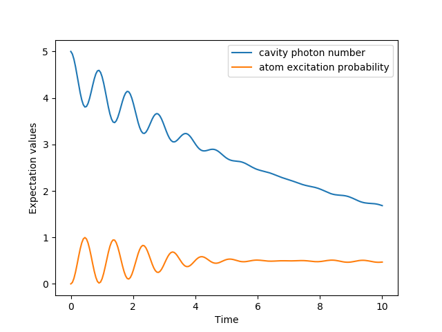
This numerical approach is precisely what's implemented in libraries like QuTiP (Quantum Toolbox in Python). For a future project, you won't need to build the Liouvillian by hand. You would simply define your Hamiltonian and a list of your collapse operators ($\sqrt{{\gamma }_k}{L}_k$), and QuTiP's mesolve (master equation solver) will handle the rest.

Conclusion

Today we have bridged the gap from the static description of quantum states to the dynamic evolution of systems interacting with their environment.

Key Takeaways:

• Real quantum systems are open, and their interaction with an environment leads to dissipation (energy loss) and decoherence (loss of phase information).
• The Lindblad master equation is the fundamental equation describing the time evolution of a system's density matrix under the Born, Markov, and Rotating Wave approximations.
• It consists of a unitary part (from the Hamiltonian $H$) and a dissipative part, the Lindbladian, which is built from jump operators $L_k$ that model specific physical processes like decay or dephasing.
• For numerical solutions, the Lindblad equation is typically converted into a matrix-vector ODE by constructing a Liouvillian superoperator, which can then be solved using standard numerical techniques.

Preview of the Next Lesson:
We will continue our exploration of open quantum systems by analyzing a canonical model in detail: a two-level system coupled to a thermal bath. This will allow us to explicitly see how temperature enters the master equation, how the system evolves towards a thermal equilibrium state, and to formally define the relaxation ($T_1$) and dephasing ($T_2$) times. This is a cornerstone model for understanding quantum effects in solid-state and atomic systems.