Random Forests vs. Gradient Boosting: Bias, Variance, and Training

Introduction

In our previous lessons, we explored the two dominant paradigms of tree-based ensemble learning. First, we examined Random Forests, which build many deep decision trees in parallel on bootstrapped data subsets to reduce variance. Then, we delved into Boosting, a sequential method where each new, simple model is trained to correct the errors of its predecessors, primarily to reduce bias.

Today, we will synthesize this knowledge to conduct a direct and rigorous comparison between Random Forests and Gradient Boosting. Our goal is to dissect their fundamental differences in training procedures and analyze how these differences lead to distinct behaviors concerning the bias-variance tradeoff. Understanding this contrast is crucial for making informed modeling decisions, as it dictates everything from hyperparameter tuning strategies to computational scalability and final predictive performance.

Comparing the Training Philosophies

At a high level, the structural difference between Random Forests and Gradient Boosting is one of parallel versus sequential construction. This distinction in their training architecture is the root cause of all their other differing characteristics.

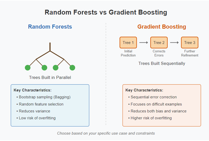
Let's formalize this distinction:

• Random Forests: Parallel De-correlation. A Random Forest trains a large number of deep decision trees independently. Each tree is trained on a different bootstrap sample of the data. Crucially, at each split in a tree, only a random subset of features is considered. This two-fold randomization—of data and features—aims to produce trees that are as uncorrelated as possible. The final prediction is a simple average (for regression) or majority vote (for classification) of all the individual tree predictions. This is an exercise in "wisdom of the crowd," where averaging many independent, noisy estimates yields a stable, low-variance result.

• Gradient Boosting: Sequential Error Correction. Gradient Boosting builds an ensemble one tree at a time. The first tree is fit to the data, and its errors (residuals) are calculated. The second tree is not fit to the original data, but rather to these residuals. Its goal is to model the error of the first tree. This process continues iteratively: each new tree is fit to the remaining error of the current ensemble. The final model is an additive combination of all the trees, with each new tree's contribution scaled by a small learning rate. This is a process of "focused improvement," where the model gradually refines its predictions by sequentially correcting its own mistakes.

This video from the MLVU course provides an excellent intuitive recap of both bagging (the basis of Random Forests) and boosting.

Dissecting the Bias-Variance Tradeoff

The different training philosophies of Random Forests and Gradient Boosting represent two distinct strategies for navigating the bias-variance tradeoff. To frame this, let's use the classic dartboard analogy:

• Bias is a measure of systematic error. A high-bias model consistently misses the bullseye in the same direction.
• Variance is a measure of inconsistency. A high-variance model's shots are scattered all over the board, even if their average is centered on the bullseye.

The MLVU video offers a fantastic introduction to this concept.

With this framework, we can now analyze how each method tackles error.

Random Forest: A Variance Reduction Strategy

A Random Forest is built from individual decision trees that are intentionally grown deep, with minimal pruning. A single deep tree is a low-bias, high-variance model; it can perfectly capture the training data (low bias) but is highly sensitive to small changes in that data (high variance).

Random Forest's strategy is to attack the variance term directly. The final prediction is an average of $B$ trees. If the predictions of these trees were independent, the variance of the ensemble would be ${\sigma }^2/B$, where ${\sigma }^2$ is the variance of a single tree. However, since the trees are trained on subsets of the same data, their predictions are correlated with a correlation $\rho$. The variance of the averaged ensemble is actually:

$$\text{Var}({\hat{f}}_{\text{RF}})=\rho {\sigma }^2+\frac{1-\rho }{B}{\sigma }^2$$

This formula reveals the entire strategy. By randomly selecting features at each split, Random Forest actively tries to reduce the correlation $\rho$ between the trees. As $B$ grows, the second term vanishes, and the overall variance is limited by $\rho {\sigma }^2$. By making the trees as independent as possible, Random Forest dramatically reduces the variance of the high-variance base learners, resulting in a strong, stable model.

Gradient Boosting: A Bias Reduction Strategy

Gradient Boosting takes the opposite approach. It uses high-bias, low-variance base learners—typically very shallow trees (sometimes just stumps with a single split). A single shallow tree is a weak learner; it has low variance but cannot capture complex patterns in the data (high bias).

Gradient Boosting's strategy is to sequentially reduce bias. By fitting each new tree to the residuals of the current ensemble, it incrementally learns the part of the signal that the existing model is missing. It chips away at the bias, step-by-step. The learning rate $\nu$ (or shrinkage) plays a crucial regularization role, preventing the model from correcting the bias too quickly and thus increasing variance excessively.

As boosting iterations proceed, the model's complexity grows, bias decreases, and variance slowly increases. This process is a form of functional gradient descent.

Practical Implications and Performance

The theoretical differences in training and bias-variance strategy lead to important practical consequences.

Tuning and Overfitting

• Random Forest: It is remarkably resistant to overfitting. Since the core mechanism is averaging, adding more trees generally does not increase the test error. The performance simply converges. The primary hyperparameters to tune are the number of features to consider at each split (mtry) and the maximum depth of the trees.
• Gradient Boosting: It can easily overfit if too many trees are added. The ensemble can begin to model the noise in the residuals. Therefore, the number of trees is a critical tuning parameter that must be determined via cross-validation. Other key parameters are the tree depth (interaction depth) and the learning rate. There is a direct tradeoff between the number of trees and the learning rate: a smaller learning rate requires more trees to achieve the same performance but often results in a better final model.

The Stanford Online video provides an excellent summary of the tuning parameters in boosting.

The following graph from an empirical study on a gene expression dataset illustrates this.

Computational Considerations

Your background in computer science makes the computational distinction particularly clear:

• Random Forest is embarrassingly parallel. Since each tree is built independently, you can distribute the training of the forest across multiple CPU cores or even multiple machines with near-linear speedup.
• Gradient Boosting is inherently sequential. The training of tree $B$ cannot begin until tree $B-1$ is complete. While the construction of a single tree can be parallelized, the overall ensemble construction is a serial process.

Relative Performance

Both methods are considered state-of-the-art for tabular data. Which performs better is problem-dependent.

• Gradient Boosting often has a slight edge in raw predictive accuracy, especially in competitions like Kaggle. Its ability to focus on hard examples allows it to capture very fine-grained patterns in the data.
• Random Forest is often easier to tune and more robust. It's a fantastic first-choice model because it provides strong performance with less hyperparameter optimization.

One study found that Random Forest excels at handling data with sharp discontinuities, while Gradient Boosting is stronger for capturing smooth, continuous patterns.

Summary of Differences

Feature	Random Forest	Gradient Boosting
Training Procedure	Parallel: Builds independent trees on bootstrap samples.	Sequential: Builds one tree at a time to correct prior errors.
Base Learners	Deep trees (low bias, high variance).	Shallow trees (high bias, low variance).
Primary Goal	Reduce variance by averaging de-correlated trees.	Reduce bias by sequentially modeling residuals.
Overfitting	Very robust. Performance converges as more trees are added.	Can overfit. The number of trees is a critical tuning parameter.
Hyperparameters	mtry (features per split), tree depth. Less sensitive to number of trees.	Learning rate, number of trees, tree depth. Performance is sensitive to all three.
Computation	Embarrassingly parallel.	Inherently sequential.

Conclusion

We have now completed our comparative analysis of Random Forests and Gradient Boosting. You should now have a firm grasp of their distinct theoretical underpinnings and practical behaviors.

Key takeaways from this lesson are:

• Random Forest builds a "forest" of deep, independent trees in parallel and averages their predictions. This is a powerful variance reduction technique.
• Gradient Boosting builds an "assembly line" of shallow trees sequentially, where each tree corrects the errors of the preceding ones. This is a powerful bias reduction technique.
• This core difference dictates their sensitivity to overfitting, their tuning strategies, and their computational characteristics. Random Forest is robust and parallelizable, while Gradient Boosting is often slightly more performant but requires careful tuning and is inherently serial.

With this, we conclude our in-depth study of tree-based ensemble methods. In the next lesson, we will pivot to an entirely different and powerful classification algorithm: the Support Vector Machine (SVM). Instead of partitioning the feature space with trees, SVMs approach classification from a geometric perspective, seeking to find the optimal separating hyperplane between classes.