Maximum-Margin Classification: The SVM Principle

Recommended resources

The freely available resources this lesson will direct you to.

Introduction

In our last lesson, we concluded our study of tree-based ensemble methods by comparing Random Forests and Gradient Boosting, focusing on their distinct approaches to managing the bias-variance tradeoff. We saw how both methods, despite their power, fundamentally operate by recursively partitioning the feature space.

Today, we shift our perspective entirely. We will introduce a new and powerful class of models, Support Vector Machines (SVMs), which approach classification not through partitioning, but through geometry. The central idea of an SVM is to find an optimal separating boundary, or hyperplane, between classes. Our primary goal is to derive the foundational principle of SVMs: maximum-margin classification. We will formalize the intuition of finding the "best" decision boundary and translate it into a constrained optimization problem. By solving this problem, we will uncover the core mechanics of SVMs and the crucial role of support vectors.

From Intuition to a Formal Problem: The Widest Street

Imagine a set of data points belonging to two different classes in a feature space. If these classes are linearly separable, there are infinitely many straight lines (or hyperplanes in higher dimensions) that could serve as a decision boundary. Which one is best?

Intuitively, the most robust boundary would be the one that is as far as possible from the data points of both classes. This provides the largest possible "cushion" before a new data point is misclassified. An SVM formalizes this intuition by seeking to find the hyperplane that maximizes this cushion, or margin. This is often visualized as finding the "widest street" that separates the two classes, where the "gutters" of the street are defined by the data points closest to the boundary.

Professor Patrick Winston's lecture from MIT OpenCourseWare provides an excellent, step-by-step development of this core idea.

16. Learning: Support Vector Machines

This video introduces the foundational concept of SVMs as finding the "widest street" to separate data points. It's a highly intuitive starting point before we dive into the formal mathematics.

Please watch the segment from Well, it's all about decision boundaries, where the "widest street" analogy is introduced and contrasted with other classifiers.

Formalizing the Margin

To turn this intuition into a solvable problem, we need to define the margin mathematically. We'll start by defining our linear classifier and then introduce two related concepts: the functional margin and the geometric margin.

Let our hyperplane be defined by the equation $w^{T} x + b = 0$ , where $w$ is the normal vector to the hyperplane and $b$ is a bias term. For a given data point $(x_{i}, y_{i})$ with $y_{i} \in {- 1, + 1}$ , we can make a prediction based on the sign of $w^{T} x_{i} + b$ .

Functional and Geometric Margin

The functional margin of a single data point $(x_{i}, y_{i})$ with respect to the hyperplane $(w, b)$ is defined as:
$γ^_{i} = y_{i} (w^{T} x_{i} + b)$
A large positive functional margin means we are making a correct and confident prediction. However, as Professor Andrew Ng points out, we can arbitrarily increase the functional margin by simply scaling $w$ and $b$ (e.g., replacing them with $2 w$ and $2 b$ ) without changing the decision boundary itself.

To get a meaningful, scale-invariant measure, we define the geometric margin, which is the actual Euclidean distance from the point $x_{i}$ to the hyperplane.

A hyperplane defined by $\theta^T x + \theta_0 = 0$ (equivalent to our $\mathbf{w}^T\mathbf{x} + b = 0$). The geometric margin $\gamma^{(i)}$ for a point $x^{(i)}$ is the perpendicular distance to the hyperplane.

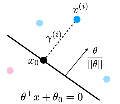
The geometric margin for a point $x_{i}$ is given by:
$γ_{i} = \frac{y _{i} ( w ^{T} x _{i} + b )}{∥ w ∥} = \frac{γ ^ _{i}}{∥ w ∥}$
This quantity is invariant to the scaling of $w$ and $b$ . Our goal is to maximize the geometric margin for the data point closest to the hyperplane. This leads to the maximum margin classifier.

Professor Ng's lecture provides a clear and concise explanation of these two types of margins.

Lecture 6 - Support Vector Machines | Stanford CS229: Machine Learning Andrew Ng (Autumn 2018)

This video formalizes the concepts of functional and geometric margin, which are crucial for setting up the SVM optimization problem.

Watch the segment on the functional margin from All right so let's start developing. Pay attention to how it captures classification confidence and its weakness to parameter scaling. Next, watch the explanation of the geometric margin from in a little bit. Okay. This section derives the geometric margin as the normalized functional margin and poses the initial optimization problem.

The Primal Optimization Problem

We want to find the parameters $w$ and $b$ that maximize the geometric margin with respect to the entire training set, which we define as $γ = min_{i} γ_{i}$ . This can be formulated as:
$max_{w, b} γ subject to \frac{y _{i} ( w ^{T} x _{i} + b )}{∥ w ∥} \geq γ, \forall i$
This problem is difficult to solve directly. We can simplify it by leveraging the scaling property of the functional margin. Let's fix the functional margin of the support vectors (the points on the "gutters") to 1. That is, for the points closest to the hyperplane, we set $γ^= min_{i} γ^_{i} = 1$ .

This implies that $γ = \frac{γ ^}{∥ w ∥} = \frac{1}{∥ w ∥}$ . Maximizing $γ$ is therefore equivalent to minimizing $∥ w ∥$ , or, for mathematical convenience, minimizing $\frac{1}{2} ∥ w ∥^{2}$ .

The constraint $y_{i} (w^{T} x_{i} + b) \geq 1$ must now hold for all data points. This transforms our problem into a standard quadratic programming (QP) form:

Primal SVM Problem (Hard Margin):

w, b min \frac{1}{2} ∥ w ∥^{2} subject to y_{i} (w^{T} x_{i} + b) \geq 1, i = 1, \dots, N

The following reading from Bishop's Pattern Recognition and Machine Learning provides the formal derivation we just outlined.

7.1. Maximum Margin Classifiers

This text provides a rigorous, step-by-step derivation of the primal optimization problem for SVMs.

Read the introduction and the section that follows, from the initial setup up to the canonical representation. Then, continue reading the formulation of the quadratic programming problem.

Solving via Lagrange Duality: The Dual Problem

This is a constrained optimization problem, a perfect scenario for using Lagrange multipliers. Since your background includes advanced mathematics, the application of this technique should be familiar. We introduce a Lagrange multiplier $α_{i} \geq 0$ for each constraint. The Lagrangian function is:
$L (w, b, α) = \frac{1}{2} ∥ w ∥^{2} - \sum_{i = 1}^{N} α_{i} (y_{i} (w^{T} x_{i} + b) - 1)$
To find the solution, we minimize $L$ with respect to $w$ and $b$ and maximize it with respect to $α$ . We start by setting the partial derivatives with respect to $w$ and $b$ to zero:

$\frac{\partial L}{\partial w} = w - \sum_{i = 1}^{N} α_{i} y_{i} x_{i} = 0 ⟹ w = \sum_{i = 1}^{N} α_{i} y_{i} x_{i}$
$\frac{\partial L}{\partial b} = - \sum_{i = 1}^{N} α_{i} y_{i} = 0 ⟹ \sum_{i = 1}^{N} α_{i} y_{i} = 0$

The first condition is remarkable: it shows that the optimal weight vector $w$ is a linear combination of the input data vectors $x_{i}$ .

Substituting these conditions back into the Lagrangian eliminates $w$ and $b$ , yielding the Wolfe dual optimization problem:

Dual SVM Problem:

α max W (α) = i = 1 \sum N α_{i} - \frac{1}{2} i = 1 \sum N j = 1 \sum N α_{i} α_{j} y_{i} y_{j} (x_{i}^{T} x_{j}) subject to α_{i} \geq 0 and i = 1 \sum N α_{i} y_{i} = 0

This dual formulation is also a QP problem. Its advantage is that the data points appear only through dot products $x_{i}^{T} x_{j}$ . This is the key that will unlock the "kernel trick" in our next lesson.

Support Vectors and the KKT Conditions

The solution to this constrained optimization problem must satisfy the Karush-Kuhn-Tucker (KKT) conditions. A key KKT condition is complementary slackness, which states that for each data point:
$α_{i} (y_{i} (w^{T} x_{i} + b) - 1) = 0$
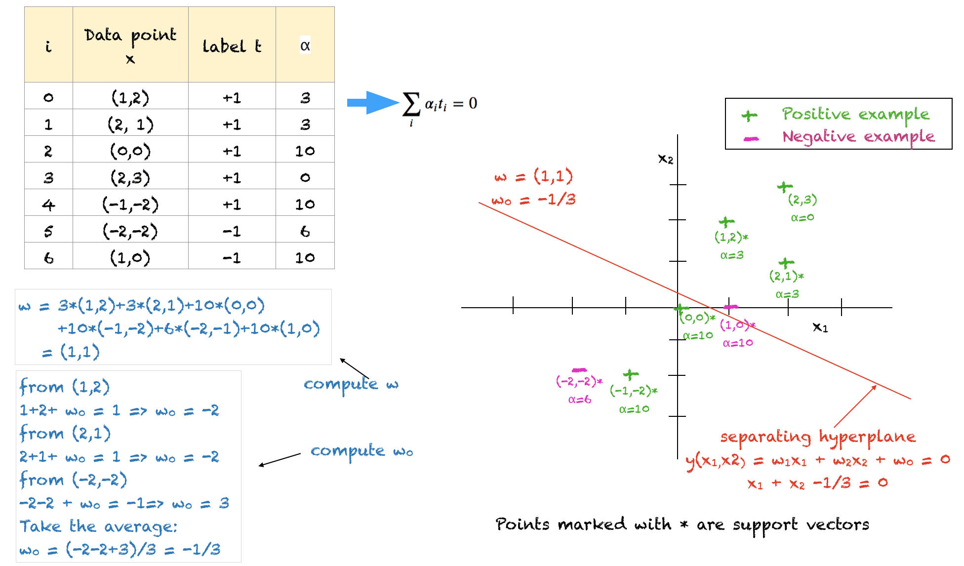
This condition implies that for any given data point $i$ , either:

$α_{i} = 0$ : The point is correctly classified and lies outside the margin ( $y_{i} (w^{T} x_{i} + b) > 1$ ). These points do not contribute to the definition of the hyperplane $w$ .
$α_{i} > 0$ : The point lies exactly on the margin boundary ( $y_{i} (w^{T} x_{i} + b) = 1$ ). These are the support vectors.

This is a crucial property of SVMs: the optimal hyperplane is determined only by the support vectors. The model is sparse in the sense that most $α_{i}$ will be zero, and only a small subset of the data defines the decision boundary.

An example of an SVM calculation. The separating hyperplane is determined by the three support vectors (marked with asterisks), which have non-zero Lagrange multipliers ($\alpha_i > 0$). The weight vector $\mathbf{w}$ is a linear combination of these support vectors, and the bias $w_0$ (our $b$) is calculated from them.

The following reading provides the derivation of the dual problem and explains the role of the KKT conditions and support vectors.

7.1. Maximum Margin Classifiers

This part of the text details the use of Lagrange multipliers to derive the dual formulation and explains the concept of support vectors through the KKT conditions.

Read the sections from the introduction of Lagrange multipliers to the final prediction equation. Then, continue with the section on KKT conditions and support vectors.

A Deeper Geometric View: Convex Hulls

There is another, highly elegant geometric interpretation of this duality. Maximizing the margin between the two classes is equivalent to finding the two closest points in the convex hulls of each class. The optimal hyperplane is the perpendicular bisector of the line segment connecting these two points.

The primal problem (maximizing the margin) and the dual problem (finding the closest points between convex hulls) are two sides of the same coin. For linearly inseparable data, this extends to finding the closest points between "reduced" convex hulls, which contract away from outliers. This perspective gives a clear geometric meaning to the optimization process and the parameters involved.

[PDF] Duality and Geometry in SVM Classifiers

This paper provides a powerful geometric interpretation of SVM duality, connecting the max-margin problem to finding the closest points between convex hulls.

First, read Section 2, "Geometric Intuition: Separable Case", to understand the core idea. Notice how it formulates two optimization problems: C-Hull (finding closest points) and C-Margin (maximizing distance between supporting planes). Then, skim the mathematical transformations in the rest of the section starting from the equivalence claim. Finally, read the first paragraph of Section 4, "Equivalence to Classic Formulation", and Theorem 4.1. This section formally proves that the C-Hull problem is the dual of the C-Margin problem, solidifying the geometric intuition with mathematical rigor.

From Hard to Soft Margin: Handling Non-Separable Data

The derivation so far assumes the data is perfectly linearly separable. In practice, this is rarely the case due to noise or overlapping class distributions. To handle this, we relax the "hard" margin constraint $y_{i} (w^{T} x_{i} + b) \geq 1$ into a soft margin.

We introduce non-negative slack variables $ξ_{i} \geq 0$ for each data point. The constraint becomes:
$y_{i} (w^{T} x_{i} + b) \geq 1 - ξ_{i}$

If $ξ_{i} = 0$ , the point is correctly classified and on or outside the margin.
If $0 < ξ_{i} \leq 1$ , the point is inside the margin but still on the correct side of the decision boundary.
If $ξ_{i} > 1$ , the point is misclassified.

We add a penalty term to the objective function to minimize the total amount of slack:
$min_{w, b, ξ} \frac{1}{2} ∥ w ∥^{2} + C \sum_{i = 1}^{N} ξ_{i}$
The parameter $C > 0$ is a regularization hyperparameter that controls the tradeoff between maximizing the margin (low $∥ w ∥^{2}$ ) and minimizing the classification error (low $\sum ξ_{i}$ ). A large $C$ heavily penalizes errors, approaching the hard-margin solution, while a small $C$ allows for a wider margin at the cost of more margin violations.

The dual formulation for the soft-margin SVM is very similar to the hard-margin case, with the only change being an upper bound on the Lagrange multipliers: $0 \leq α_{i} \leq C$ .

This brief introduction to the soft margin is crucial, as it is the formulation used in practice and the one that is extended by the kernel trick.

7.1. Maximum Margin Classifiers

This final reading introduces the soft-margin SVM by incorporating slack variables to handle non-separable data.

Read the entire section on "Overlapping class distributions". This will show you how the optimization problem is modified with slack variables and the penalty parameter C.

Conclusion

In this lesson, we have laid the theoretical groundwork for Support Vector Machines. We moved from the simple intuition of finding the "widest street" to a formal, constrained optimization problem.

The key takeaways are:

The maximum-margin principle provides a geometric and theoretically sound basis for finding an optimal linear classifier.
This principle can be formulated as a quadratic programming problem that seeks to minimize $∥ w ∥^{2}$ while ensuring all data points are correctly classified outside a margin.
Using Lagrange duality, we derived the dual formulation, which depends only on the dot products of data vectors.
The solution is sparse and relies on a subset of data points called support vectors, which lie on the margin boundaries and have non-zero Lagrange multipliers $α_{i}$ .
For non-separable data, the soft-margin formulation introduces slack variables and a regularization parameter $C$ to control the bias-variance tradeoff between margin width and classification error.

We have now derived the linear SVM. However, its true power lies in its ability to create non-linear decision boundaries. In our next lesson, we will explore the kernel trick, a profound idea that leverages the dual formulation to project data into high-dimensional feature spaces implicitly, allowing SVMs to learn highly complex, non-linear classifiers efficiently.