The Kernel Trick Explained

Recommended resources

The freely available resources this lesson will direct you to.

Introduction

In our last lesson, we delved into the mechanics of Support Vector Machines, deriving the maximum-margin principle and formulating it as a constrained optimization problem. The crucial step was our transition to the dual formulation, which revealed a remarkable property: the entire optimization, and subsequent predictions, depend only on the inner products of data vectors, $x_{i}^{T} x_{j}$ . We concluded by noting that this specific structure is the key to unlocking the true power of SVMs.

Today, we will build directly on that foundation to explore the kernel trick. This elegant and powerful concept addresses the primary limitation of the linear SVM we derived: its inability to handle non-linear relationships. You will learn how the kernel trick allows SVMs to create highly complex, non-linear decision boundaries. Critically, we will see how this is achieved without ever explicitly performing the computationally expensive feature transformations that would otherwise be necessary, enabling us to work efficiently in even infinite-dimensional spaces.

From Linear to Non-Linear Separation

A linear classifier, by definition, finds a linear decision boundary—a line, a plane, or a hyperplane. This is effective when the data is linearly separable, but many real-world problems are not so clean. Consider the dataset below, where one class of points is nested inside another.

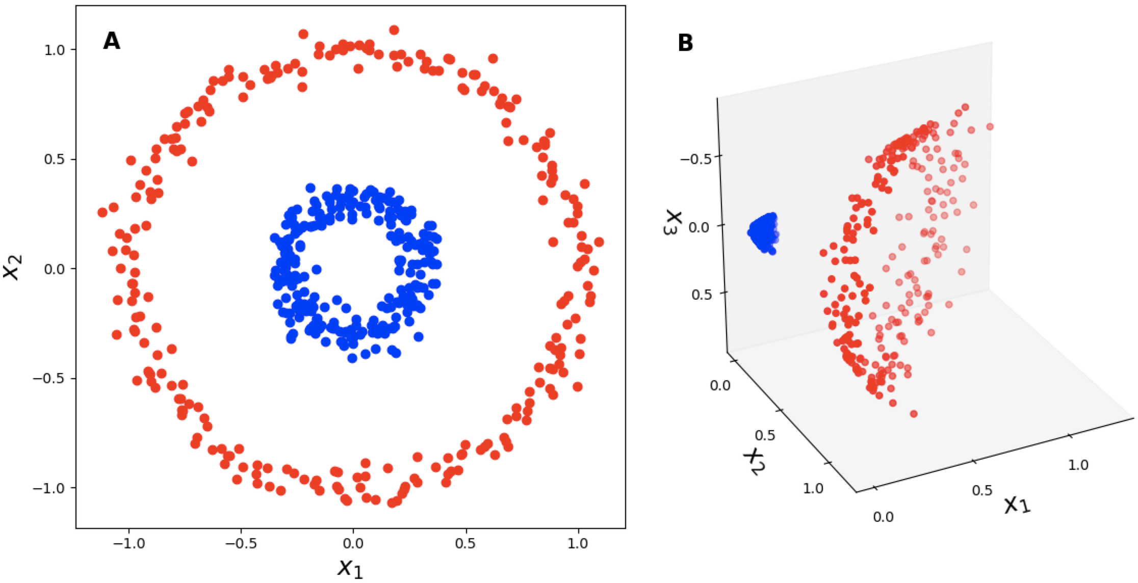
Panel A shows a 2D dataset where blue and red points are not separable by a straight line. Panel B shows the same data transformed into a 3D space, where a simple plane can now separate the two classes.

No single line in the 2D space of Panel A can separate the red and blue points. However, the core idea behind kernel methods is to project the data into a higher-dimensional feature space where it does become linearly separable. Panel B illustrates this: by adding a third dimension, $x_{3}$ , which is a function of the original features $x_{1}$ and $x_{2}$ , the classes are lifted apart and can now be separated by a simple plane.

Let's formalize this. We can define a feature mapping function, $ϕ (x)$ , that transforms our data from the input space $R^{d}$ to a higher-dimensional feature space $R^{D}$ , where $D > d$ . The strategy is then to apply our linear SVM algorithm in this new feature space.

The following short visualization from a lecture by Andrew Ng provides an excellent intuition for this process.

Lecture 7 - Kernels | Stanford CS229: Machine Learning Andrew Ng (Autumn 2018)

This video clip visualizes the concept of mapping non-linearly separable data into a higher-dimensional space to achieve linear separability.

Watch the segment from how the, uh, learning algorithm. Notice how the 2D data is projected into 3D, a separating plane is found, and this plane then corresponds to a non-linear boundary back in the original 2D space.

While this idea is powerful, it presents a significant computational challenge. If the feature space is very high-dimensional (e.g., millions or even infinite dimensions), explicitly computing the new feature vectors $ϕ (x)$ for all data points would be computationally prohibitive or impossible.

The Role of the Dual Formulation

This is where our work from the previous lesson pays off. Recall the dual optimization problem for the soft-margin SVM:

α max (i = 1 \sum N α_{i} - \frac{1}{2} i = 1 \sum N j = 1 \sum N α_{i} α_{j} y_{i} y_{j} (x_{i}^{T} x_{j})) subject to 0 \leq α_{i} \leq C and i = 1 \sum N α_{i} y_{i} = 0

If we apply our feature mapping $ϕ$ , every instance of $x_{i}$ becomes $ϕ (x_{i})$ . The optimization problem then depends on the inner product in the new feature space, $ϕ (x_{i})^{T} ϕ (x_{j})$ .

Likewise, the prediction for a new point $x$ becomes:
$f (x) = sign (w^{T} ϕ (x) + b) = sign (\sum_{i = 1}^{N} α_{i} y_{i} (ϕ (x_{i})^{T} ϕ (x)) + b)$
Notice again, the only way data enters the training and prediction stages is through inner products. This is not a coincidence; it is the property that makes the kernel trick possible.

The Kernel Trick: A Computational Shortcut

The "kernel trick" is the realization that if we have a function $K (x_{i}, x_{j})$ that directly computes the result of the inner product $ϕ (x_{i})^{T} ϕ (x_{j})$ without ever forming the vectors $ϕ (x_{i})$ and $ϕ (x_{j})$ , we can gain all the benefits of working in the high-dimensional space without the computational cost. This function is called a kernel function.

The Kernel Trick: Replace every instance of the inner product $x_{i}^{T} x_{j}$ in the SVM algorithm with a kernel function $K (x_{i}, x_{j})$ .

Let's see a concrete example. Suppose our input space is $R^{n}$ and we want to use all pairwise products of features as our new feature space. For $x \in R^{n}$ , the feature vector $ϕ (x)$ would contain all terms $x_{i} x_{j}$ and would have $n^{2}$ dimensions. Explicitly computing the inner product $ϕ (x)^{T} ϕ (z)$ would take $O (n^{2})$ time.

However, consider the simple function $K (x, z) = (x^{T} z)^{2}$ .

(x^{T} z)^{2} = (i = 1 \sum n x_{i} z_{i})^{2} = i = 1 \sum n j = 1 \sum n (x_{i} x_{j}) (z_{i} z_{j}) = ϕ (x)^{T} ϕ (z)

Computing $(x^{T} z)^{2}$ involves one inner product in the original $n$ -dimensional space, which takes $O (n)$ time, and then one squaring operation. We have computed the result of an $O (n^{2})$ operation in $O (n)$ time. This is the essence of the trick.

The following video provides an excellent walkthrough of this exact example and formalizes the general recipe for applying the kernel trick.

Lecture 7 - Kernels | Stanford CS229: Machine Learning Andrew Ng (Autumn 2018)

This video details the "recipe" for applying the kernel trick and demonstrates the computational savings with a concrete example of a polynomial kernel.

First, watch the "recipe" for the kernel trick explained from machine learning people. Then, pay close attention to the detailed derivation of the polynomial kernel from let's go through one example, which shows how an O(n^2) computation is reduced to O(n).

Common Kernel Functions

By choosing different kernel functions, we can implicitly choose different high-dimensional feature spaces and thus create different types of non-linear decision boundaries. Some of the most common kernels are:

Linear Kernel: $K (x, z) = x^{T} z$ . This is simply the original linear SVM. It's useful as a baseline and when the data is already linearly separable.
Polynomial Kernel: $K (x, z) = (γ x^{T} z + r)^{d}$ . This kernel corresponds to a feature space of polynomials of degree up to $d$ . The hyperparameters $γ$ (gamma), $r$ (coefficient), and $d$ (degree) control the behavior of the mapping.
Radial Basis Function (RBF) or Gaussian Kernel: $K (x, z) = exp (- γ ∥ x - z ∥^{2})$ . This is arguably the most popular and powerful kernel. It can be interpreted as a similarity measure that is 1 when $x = z$ and decays to 0 as the points move apart. The hyperparameter $γ$ controls the "width" of the basis function; a small $γ$ creates a very broad decision region, while a large $γ$ creates a more complex, localized region.

The remarkable theoretical property of the RBF kernel is that its corresponding feature space, $ϕ (x)$ , is infinite-dimensional. The kernel trick allows us to perform classification in this infinitely complex space with finite computation.

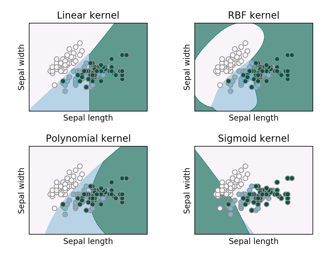
The following image shows how these different kernels affect the final decision boundary on a sample dataset.

Decision boundaries generated by SVMs with different kernel functions on the same dataset. The linear kernel produces a line, while the RBF, Polynomial, and Sigmoid kernels produce complex, non-linear boundaries.

The Theory: What Constitutes a Valid Kernel?

This raises a crucial theoretical question: can any arbitrary function $K (x, z)$ serve as a kernel? The answer is no. A function must satisfy certain mathematical properties to ensure it corresponds to a real inner product in some Hilbert space.

The key result that governs this is Mercer's Theorem. It states that a function $K$ can be a valid kernel if and only if for any finite set of points ${x_{1}, \dots, x_{N}}$ , the corresponding kernel matrix (or Gram matrix) $K$ , where $K_{ij} = K (x_{i}, x_{j})$ , is symmetric and positive semi-definite.

Why is this important? The positive semi-definite property of the kernel matrix ensures that the quadratic term in the SVM dual objective function is convex. This guarantees that the optimization problem has a unique global minimum, which is essential for a well-behaved and solvable learning algorithm. The kernel trick doesn't just provide a computational shortcut; it does so while preserving the desirable optimization properties of the SVM.

The following resources provide a more detailed and formal treatment of kernel functions and the conditions for their validity.

[PDF] Kernel Methods and SVMs Contents

This document provides a concise and mathematically rigorous overview of the kernel trick, common kernels, and the theory behind them.

First, read section 3, "The Kernel Trick", for a formal introduction. Next, read section 4, "Support Vector Machines", which shows how the SVM dual problem is "kernelized". Finally, read the beginning of section 6, "Kernel Theory", and the statement of Mercer's Theorem within it. This section formalizes the conditions for a valid kernel.

13. Kernel Methods

This video from Inside Bloomberg offers another clear, industry-focused perspective on kernel methods.

Start by watching the segment from that was when we went that reviews the dual SVM problem and highlights its "kernelized" form. Next, watch from we introduced the kernel function for an explanation of the kernel function and the computational speedup. Then, watch the summary of the kernel trick from later on okay so let me just. Finally, watch the explanation of the RBF (Gaussian) kernel from the kernel that by far, which emphasizes its role in accessing infinite-dimensional feature spaces.

Conclusion

In this lesson, we have unlocked the full potential of Support Vector Machines by introducing the kernel trick. We saw how a limitation of linear models—their inability to capture non-linear patterns—can be overcome by projecting data into a higher-dimensional space.

The key takeaways are:

The kernel trick is a method for using a linear classifier to solve a non-linear problem by implicitly mapping the data to a high-dimensional feature space.
This is possible because the SVM's dual formulation depends only on inner products of data vectors.
A kernel function $K (x, z)$ is a computationally efficient shortcut to compute the inner product $ϕ (x)^{T} ϕ (z)$ in the feature space without ever explicitly calculating the high-dimensional vectors $ϕ (x)$ .
Common kernels like the Polynomial and RBF (Gaussian) kernels allow SVMs to learn a wide variety of non-linear decision boundaries. The RBF kernel, in particular, corresponds to an infinite-dimensional feature space.
Mercer's Theorem provides the theoretical foundation, stating that a function is a valid kernel if and only if its kernel matrix is positive semi-definite, which ensures the SVM optimization problem remains convex and solvable.

This concludes our module on advanced supervised methods. You now have a theoretical understanding of powerful techniques ranging from tree ensembles to kernel-based machines. In our next module, we will pivot to an entirely new area of machine learning: unsupervised learning, where the goal is to discover hidden patterns and structures in data without the guidance of pre-existing labels. We will begin by exploring one of the most fundamental clustering algorithms, K-means.