Recommended resources
The freely available resources this lesson will direct you to.
Introduction
In our last session, we explored Bagging and Random Forests, powerful ensemble methods that operate in parallel. By training multiple independent models on bootstrapped data and averaging their predictions, they effectively reduce the variance of a single model, leading to more robust predictions.
Today, we shift our focus to a fundamentally different ensemble philosophy: Boosting. Unlike the parallel approach of Bagging, Boosting builds models sequentially. Each new model in the sequence is trained to correct the errors made by the ensemble of preceding models. This iterative, corrective process is a powerful technique for reducing model bias. Our objective is to understand the general boosting framework and then dissect and contrast the mechanisms of its two most historically significant implementations: AdaBoost and Gradient Boosting.
The General Boosting Framework: Forward Stagewise Additive Modeling
At its core, boosting is an application of a statistical concept known as additive modeling. The goal is to build a highly accurate prediction function, , by incrementally adding "weak" learners (simple models like decision stumps) to the ensemble. A weak learner is defined as a model that performs only slightly better than random guessing.
The process is greedy and sequential, often formalized as Forward Stagewise Additive Modeling. We start with an initial simple model, , and at each step , we add a new weak learner, , scaled by some factor , to minimize the overall loss function . The final model is an additive combination of all the weak learners:
At each step , the algorithm solves for the best new weak learner and its corresponding coefficient:
This general framework is the theoretical backbone of all boosting algorithms. The key differences between various boosting methods, such as AdaBoost and Gradient Boosting, lie in their choice of the loss function and the specific optimization strategy they use to find the next weak learner .
To understand this framework in more detail, please review the following section from the paper "A Comparison of Boosting Methods".
[PDF] A Comparison of Boosting Methods for Stock Market Risk Prediction
This section introduces the Forward Stagewise Additive Modeling algorithm, which provides the general mathematical structure for all boosting methods.
Please read the subsection "Forward Stagewise Additive Modeling". Pay close attention to Algorithm 2, which formalizes the iterative process of adding base learners to minimize a loss function.
Case Study 1: AdaBoost (Adaptive Boosting)
AdaBoost, short for Adaptive Boosting, was the first truly successful boosting algorithm and provides a clear, concrete implementation of the boosting principle. It works by sequentially training weak learners, typically decision stumps (decision trees with only one split), and at each step, it adaptively re-weights the data samples.
The three core ideas behind AdaBoost are best explained in the StatQuest video "AdaBoost, Clearly Explained".
This video introduces the foundational concepts of AdaBoost, contrasting it with Random Forests to highlight its unique properties.
Please watch the introductory segment from and how it's used. This will clarify the three key principles: using weak learners, giving them variable "say" in the final vote, and building them sequentially based on prior errors.
The AdaBoost Mechanism: Re-weighting and "Amount of Say"
The core mechanism of AdaBoost revolves around two key computations at each step:
- Updating Sample Weights: The algorithm maintains a weight for each training sample. Initially, all weights are equal. After a weak learner is trained, AdaBoost increases the weights of the samples that were misclassified and decreases the weights of those that were correctly classified. This forces the next weak learner to focus more on the "hard" examples that the previous learner got wrong.
- Calculating the "Amount of Say" (): Each weak learner is assigned a weight, or "amount of say" (), in the final ensemble vote. This weight is proportional to the learner's accuracy on the weighted data. A learner with a lower error gets a larger say.
The following segments from the same StatQuest video walk through these calculations with a clear, numerical example.
These segments provide a step-by-step demonstration of how AdaBoost calculates a stump's 'say', updates sample weights, and prepares for the next iteration.
First, watch how much say to understand how the total error of a stump is used to calculate its influence, \alpha. Next, watch how to modify the weights. This part is crucial as it details the formulas for increasing and decreasing sample weights based on classification outcomes and the stump's \alpha. Finally, watch the second stump to see how the new, modified weights are used to build the subsequent learner, completing the adaptive cycle.
The Mathematical View: Minimizing Exponential Loss
The elegant mechanism of AdaBoost is not just a heuristic; it can be rigorously derived as a forward stagewise algorithm that minimizes the exponential loss function:
where .
In this view, the process of finding a weak learner that minimizes the weighted classification error at each step is equivalent to selecting the learner that best helps to minimize the overall exponential loss of the ensemble. The "amount of say", , is not an arbitrary formula but is the optimal step size that minimizes this loss at each iteration.
The derivation of this optimal step size, , where is the weighted error, is a cornerstone of AdaBoost's theory. You can find this derivation in the Cornell lecture notes on Boosting.
These sections provide the mathematical derivation that connects AdaBoost's intuitive procedure to the formal optimization of the exponential loss function.
Start by reading Case Study #2: AdaBoost to see how finding the best weak learner translates to minimizing the weighted classification error. Then, review the section Finding the stepsize α. This contains the closed-form derivation for the optimal \alpha, a key theoretical result. Finally, read the sections on Re-normalization and Further analysis. This demonstrates the elegant weight update rule and proves that AdaBoost's training error decreases exponentially, a powerful guarantee.
Case Study 2: Gradient Boosting
While AdaBoost is powerful, its derivation is tied specifically to the exponential loss function, making it primarily suited for classification. Gradient Boosting generalizes this idea to any differentiable loss function, making it a flexible framework applicable to both regression and classification.
The core insight, developed by Jerome Friedman, is to reframe boosting as a numerical optimization problem in a function space. Instead of manipulating sample weights, Gradient Boosting sequentially adds new weak learners that "point" in the direction of the negative gradient of the loss function.
The Gradient Boosting Mechanism: Fitting to Pseudo-Residuals
Here's the step-by-step process:
- Initialize: Start with an initial constant prediction, usually the mean of the target variable for regression.
- Compute Pseudo-Residuals: For each sample, calculate the negative gradient of the loss function with respect to the current prediction. This vector of gradients is called the pseudo-residual. For squared-error loss, this is simply the ordinary residual (observed - predicted).
- Fit a Weak Learner: Train a new weak learner (typically a small decision tree) to predict these pseudo-residuals. The idea is that this new tree learns the "error" of the current ensemble.
- Update the Model: Add the new weak learner to the ensemble, scaled by a learning rate (also known as shrinkage). This small, constant learning rate regularizes the model, preventing any single learner from contributing too much and improving generalization.
- Iterate: Repeat steps 2-4 until a desired number of learners is reached or performance on a validation set stops improving.
The StatQuest video on Gradient Boost provides an excellent, intuitive walkthrough of this process for a regression problem.
Gradient Boost Part 1 (of 4): Regression Main Ideas
This video clearly illustrates the core mechanism of Gradient Boosting: iteratively fitting trees to the residuals (errors) of the previous prediction.
First, watch the main explanation from let's see how the most common. Focus on how the algorithm starts with an average, calculates residuals, and fits a tree to those residuals. Pay attention to the role of the learning rate. Continue watching from so let's build another tree. This segment reinforces the iterative process, showing how a second tree is built on the new residuals, taking another small step towards improving the prediction.
The Mathematical View: Gradient Descent in Function Space
The term "Gradient Boosting" comes from the fact that this procedure is analogous to performing gradient descent. In standard gradient descent, we update a parameter vector by taking a small step in the direction of the negative gradient of the loss function: .
In Gradient Boosting, the "parameter" we are optimizing is the entire prediction function . At each step, we fit a weak learner that is maximally correlated with the negative gradient of the loss, . Adding this new learner, scaled by the learning rate, is equivalent to taking a step in function space to minimize the loss.
This theoretical connection is what makes Gradient Boosting so powerful and general. You can find a formal description of this process in the following reading.
[PDF] A Comparison of Boosting Methods for Stock Market Risk Prediction
This reading formalizes the Gradient Boosting algorithm, explaining it as a gradient descent procedure in function space.
Please read the sections 2.7.4 Gradient Boosting and review "Algorithm 5: Gradient Boosting". This will solidify your understanding of how fitting a learner to the negative gradient (git) is the core of the algorithm.
Contrasting AdaBoost and Gradient Boosting
While both are boosting algorithms, their mechanisms and philosophies differ significantly. The following images provide a high-level visual summary of these differences.
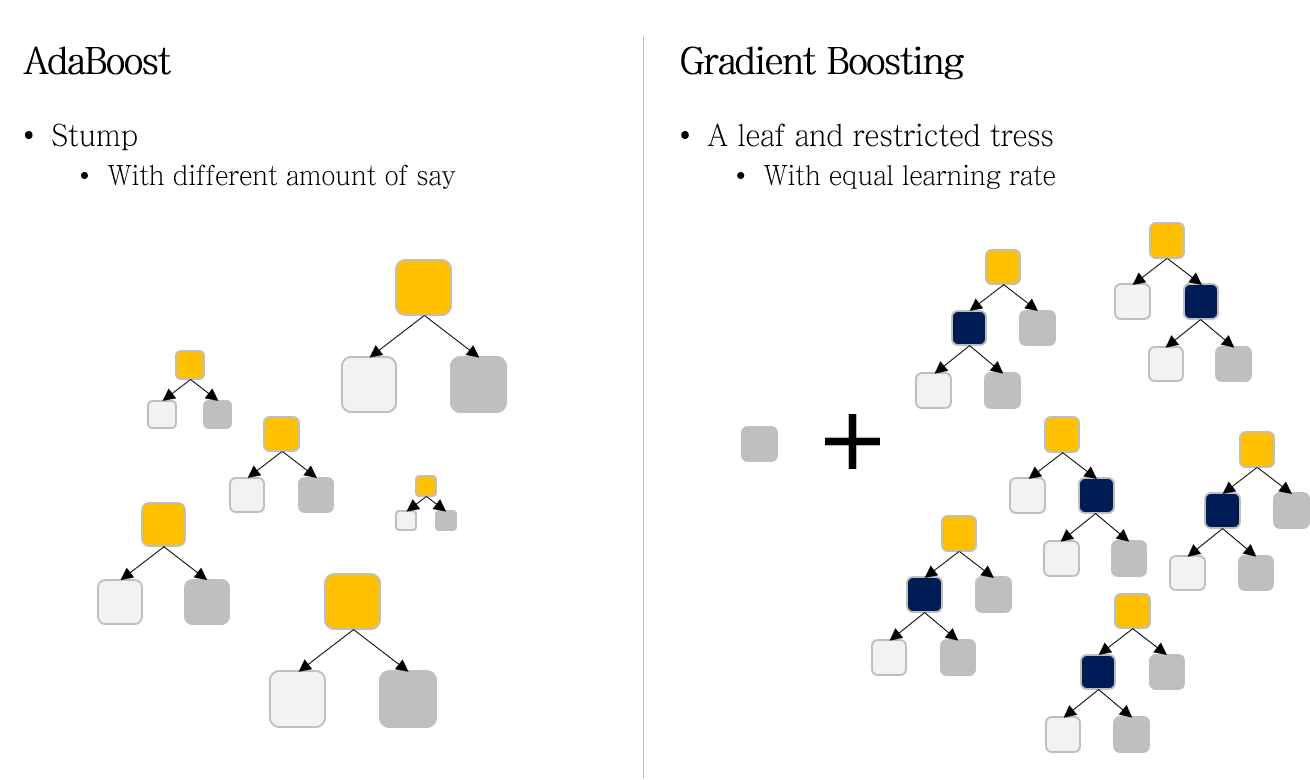
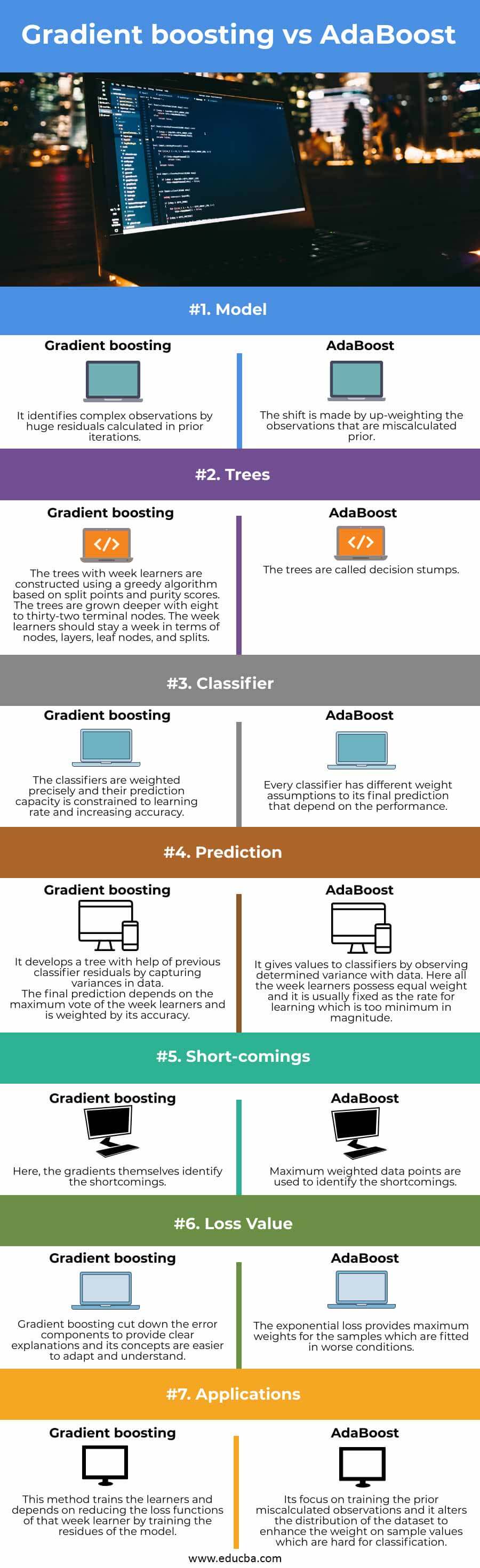
Here is a summary of the most critical distinctions:
| Feature | AdaBoost | Gradient Boosting |
|---|---|---|
| Core Idea | Adapts by increasing the weights of misclassified samples. The next learner focuses on these "hard" examples. | Generalizes boosting by treating it as a gradient descent problem. The next learner fits the negative gradient of the loss function (pseudo-residuals). |
| Loss Function | Derived from and intrinsically linked to the exponential loss function. | A general framework that works with any differentiable loss function (e.g., squared error for regression, log-loss for classification). |
| How Errors are Corrected | By increasing the weights of data points that were misclassified. | By fitting a new learner to the pseudo-residuals of the current ensemble. |
| Weak Learner's Role | Each learner is assigned a weight (, or "amount of say") based on its weighted error. The final prediction is a weighted vote. | The contribution of each new learner is scaled down by a small, constant learning rate () as a form of regularization. The final prediction is a simple sum. |
| Typical Weak Learner | Very simple models, most commonly decision stumps (a tree with one split). | Slightly more complex models, typically decision trees with a restricted number of leaves (e.g., 4 to 32). |
The paper "A Comparison of Boosting Methods" provides a concise textual summary of this comparison.
[PDF] A Comparison of Boosting Methods for Stock Market Risk Prediction
This section directly compares AdaBoost and Gradient Boosting from a theoretical standpoint, summarizing their key algorithmic differences.
Please read the first three paragraphs of section 2.8 BOOSTING METHOD COMPARISON. This text explicitly contrasts how AdaBoost updates sample weights versus how Gradient Boosting fits weak learners to the negative gradient of the loss function.
Conclusion
In this lesson, we have explored the sequential ensemble strategy of boosting. We established the general theoretical framework of Forward Stagewise Additive Modeling and then dove into the specific mechanisms of its two most foundational variants.
Key takeaways include:
- Boosting Framework: A sequential process that builds an accurate model by iteratively adding weak learners, each correcting the errors of the previous ensemble. It is primarily a bias-reduction technique.
- AdaBoost: An adaptive algorithm that works by increasing the weights of misclassified samples, forcing subsequent weak learners to focus on them. Its mechanics are mathematically equivalent to minimizing an exponential loss function.
- Gradient Boosting: A more general framework that reframes boosting as gradient descent in function space. It fits new weak learners to the pseudo-residuals (negative gradients) of any differentiable loss function, making it highly flexible.
- Core Contrast: AdaBoost corrects errors by re-weighting data, while Gradient Boosting corrects errors by modeling the gradient of the loss.
We've now covered the two dominant paradigms of tree-based ensembles: Bagging/Random Forests (parallel, variance-reducing) and Boosting (sequential, bias-reducing). In our next lesson, we will directly compare these two families, analyzing their bias-variance characteristics and typical use cases to understand when to choose one over the other.