Tensor Parallelism: Splitting Layers Across GPUs

Introduction

In our last lesson, we explored data parallelism, a technique where the entire model is replicated on each GPU to process different slices of data. We saw how this scales training throughput but is fundamentally limited by the memory of a single GPU, as every device must store the full model, its gradients, and optimizer states.

This brings us to a critical question: what happens when a model becomes so large that its parameters, or even the activations from a single layer, cannot fit into one GPU's memory?

This lesson introduces the first form of model parallelism designed to solve this problem: tensor parallelism. You will learn how this intra-layer parallelization strategy works by partitioning the weight matrices (tensors) of individual model layers across multiple GPUs. We will dissect the mathematical principles behind it and see how it is applied to the core components of a Transformer model.

1. What is Tensor Parallelism?

Tensor parallelism, also known as intra-layer model parallelism, takes a "horizontal" approach to splitting the model. Instead of assigning different layers to different GPUs (which we'll cover in the next lesson), it partitions the computation within a single, large layer.

This is a powerful technique for handling models with very "wide" layers, but it comes with a significant trade-off: it requires frequent, high-bandwidth communication between the GPUs participating in the computation.

To get a high-level overview of this concept, let's watch a brief segment from a Stanford seminar.

As the video explains, the key is to split the tensors—primarily the weight matrices—that constitute a layer. This allows all GPUs in the group to work concurrently on the same layer, avoiding the idle time or "bubble" that we will see in other model parallelism techniques. However, it necessitates communication to combine the partial results. This makes tensor parallelism highly effective but typically limited to GPUs within a single server connected by ultra-fast interconnects like NVLink.

2. The Mathematical Foundation: Parallelizing Matrix Multiplication

Modern neural networks, especially Transformers, are computationally dominated by General Matrix-Matrix Multiplications (GEMM) within their linear layers. Therefore, parallelizing a layer boils down to parallelizing its matrix multiplications.

Let's consider a linear layer's core operation: $Y=XA$, where $X$ is the input and $A$ is the weight matrix. There are two fundamental ways to partition this computation.

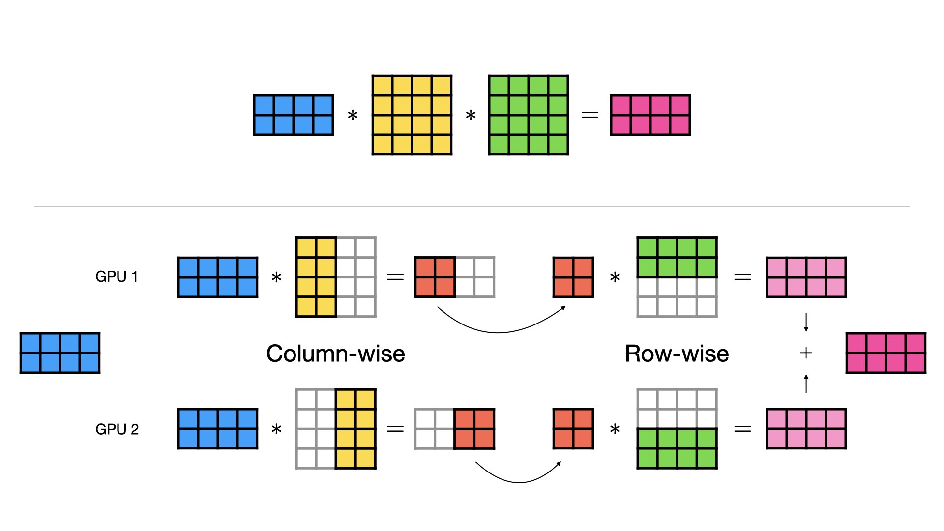
Let's summarize the two strategies from the reading:

1. Column-wise Parallelism:

   • The weight matrix $A$ is split along its columns: $A=[A_1|A_2]$.
   • The input matrix $X$ is duplicated (replicated) across all GPUs.
   • Each GPU computes a part of the output: GPU 1 computes $Y_1=X{A}_1$, GPU 2 computes $Y_2=X{A}_2$.
   • The final output $Y=[Y_1|Y_2]$ is now sharded across the GPUs. Importantly, no communication is needed to produce this sharded output.

2. Row-wise Parallelism:

   • The weight matrix $A$ is split along its rows: $A=\left(\begin{array}{c}{A}_1\\ A_2\end{array}\right)$.
   • The input matrix $X$ must also be sharded along its columns: $X=[X_1|X_2]$.
   • Each GPU computes a partial result: GPU 1 computes $Y_1=X_1{A}_1$, GPU 2 computes $Y_2=X_2{A}_2$.
   • The final output is the sum of these partial results: $Y=Y_1+Y_2$. This requires an All-Reduce collective operation to sum the partial results from all GPUs and distribute the final, replicated output to all of them.

This distinction is the key to designing efficient tensor-parallel layers. A column-parallel layer takes a replicated input and produces a sharded output. A row-parallel layer takes a sharded input and produces a replicated output.

3. Application to Transformer Blocks

The real power of tensor parallelism emerges when these strategies are chained together to parallelize a standard Transformer block, which consists of a Multi-Layer Perceptron (MLP) or Feed-Forward Network (FFN) and a Multi-Head Attention (MHA) module. The Megatron-LM paper introduced a canonical pattern for this.

The MLP / FFN Block

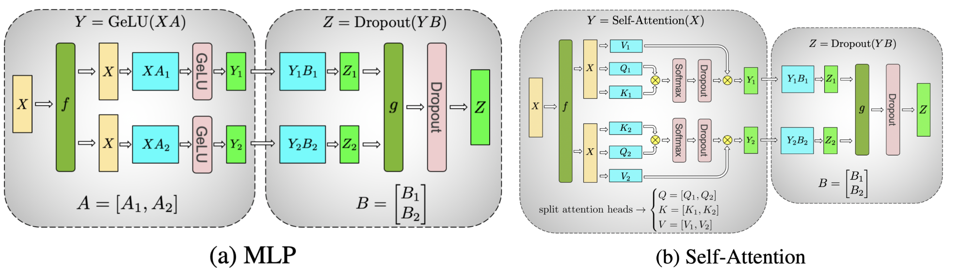
A typical MLP block looks like this: $O=\text{GeLU}(XA)B$. It consists of two linear layers with a non-linear activation function in between.

1. First Linear Layer ($XA$): This layer is implemented with column-wise parallelism. The weight matrix $A$ is split by columns. It takes the replicated input $X$ and produces a sharded intermediate activation, $Y=\text{GeLU}(XA)$.

2. Activation Function (GeLU): A critical insight is that element-wise operations like GeLU can be applied directly to the sharded output $Y$ on each GPU independently, without any need for communication. This is possible only because the first layer was column-parallel. If it were row-parallel, we would have partial sums that, after a non-linearity, would not equal the correct global result. For example, $\text{ReLU}(a+b)\ne \text{ReLU}(a)+\text{ReLU}(b)$.

3. Second Linear Layer ($YB$): This layer is implemented with row-wise parallelism. Its input $Y$ is already sharded from the previous step. The weight matrix $B$ is split by rows. Each GPU computes a partial output, and an All-Reduce is performed at the end to sum these partial outputs into the final, replicated tensor $O$.

This ColumnParallel -> RowParallel pattern is incredibly efficient because it avoids any communication between the two linear layers. It requires only one All-Reduce operation in the forward pass for the entire block.

The following resource provides a brilliant, illustrated deep-dive into this exact mechanism.

The Multi-Head Attention (MHA) Block

As the reading explains, the same ColumnParallel -> RowParallel pattern applies beautifully to the MHA block.

• The Q, K, and V projections are performed by a single large column-parallel linear layer. This naturally splits the attention heads across the GPUs.
• The scaled dot-product attention is then computed entirely locally on each GPU for its assigned heads, requiring no communication.
• The final output projection is a row-parallel linear layer that aggregates the results from the individual heads, followed by an All-Reduce to produce the replicated output tensor.

Conclusion

In this lesson, we have deconstructed tensor parallelism, moving from its high-level concept to the specific mathematical operations and design patterns that make it work.

Key Takeaways:

• Tensor Parallelism (TP) is an intra-layer strategy that partitions a model's weight matrices to distribute the computation of a single large layer across multiple GPUs.
• It is essential for models whose layers are too wide to fit in a single GPU's memory.
• The core mechanism relies on two sharding strategies for matrix multiplication:
  • Column-wise Parallelism: Produces a sharded output from a replicated input, with no communication.
  • Row-wise Parallelism: Produces a replicated output from a sharded input, requiring an All-Reduce to sum partial results.
• The canonical "Megatron" pattern pairs a ColumnParallelLinear layer with a RowParallelLinear layer. This minimizes communication by ensuring the output sharding of the first layer matches the input sharding requirement of the second, requiring only one All-Reduce per block.
• Due to its high communication frequency, TP is most effective within a single node over high-bandwidth interconnects like NVLink.

Preview of the Next Lesson:

Tensor parallelism is excellent for wide layers, but its communication overhead limits how many GPUs you can efficiently add to a tensor-parallel group. What if your model is not just wide, but also extremely deep? In our next lesson, we will explore pipeline parallelism, a complementary strategy that splits the model vertically by assigning different layers to different GPUs, creating a multi-stage pipeline. This approach introduces a different set of challenges and trade-offs, most notably the "pipeline bubble."