Pipeline Parallelism Explained

Introduction

In our previous lesson, we investigated tensor parallelism, an intra-layer strategy that partitions the computation within a single large model layer across multiple GPUs. We saw that it's highly effective for very "wide" models but is communication-intensive, making it best suited for GPUs within a single, tightly-connected node.

This leads to a natural follow-up question: what if our model is not just wide, but also exceptionally deep? This is common with modern architectures like large Transformers. In this scenario, even a single layer's activations might be manageable, but the entire stack of layers exceeds the memory of any single GPU.

Today's lesson addresses this challenge by introducing pipeline parallelism. You will learn how this inter-layer parallelization strategy works by partitioning the model's layers between a series of devices, creating a computational pipeline. We will explore how models are partitioned this way and uncover the fundamental efficiency problem this approach creates—the "pipeline bubble"—along with the standard technique used to solve it.

1. What is Pipeline Parallelism?

Pipeline parallelism, also known as inter-layer model parallelism, takes a "vertical" approach to distributing a model. Instead of splitting individual tensors within a layer, it assigns entire, consecutive blocks of layers to different devices. Think of it as an assembly line for a neural network: each GPU is a station responsible for a specific part of the overall computation. A mini-batch of data enters at the first GPU, which computes its assigned layers and passes the intermediate output (the activations) to the next GPU in the line, and so on.

The image below provides a clear visual distinction between the intra-operator parallelism we saw last lesson and the inter-operator parallelism we are discussing today.

To formalize this, let's explore how a simple model is partitioned and how data flows during the forward and backward passes.

As the reading describes, a model like $\text{output}=\text{L}\_4(\text{L}\_3(\text{L}\_2(\text{L}\_1(\text{input}))))$ can be split so that GPU1 handles layers L1 and L2, and GPU2 handles L3 and L4. The key communication steps are:

1. Forward Pass: GPU1 sends the activations from L2 to GPU2.
2. Backward Pass: GPU2 sends the gradients with respect to L2's output back to GPU1.

Notice that this requires only point-to-point communication (sending from one specific GPU to another) rather than the complex collective communication (like All-Reduce) needed for tensor parallelism. This is a major advantage, as point-to-point transfers are generally less expensive, especially across different server nodes.

However, if you look closely at the execution timeline described, you might spot a significant inefficiency.

2. The Inefficiency of Naive Pipelining: The "Bubble"

The assembly line analogy for pipeline parallelism has a flaw. In a real assembly line, all stations work simultaneously on different products. In the naive model parallelism we just reviewed, only one GPU is active at any given moment. While GPU2 is computing its forward pass, GPU1 sits idle, waiting for the backward pass to begin. This period of inactivity is a critical performance bottleneck known as the pipeline bubble.

The following video and image illustrate this problem very clearly.

The visualization in the video is conceptually identical to the one below, which shows the execution for a single, large batch.

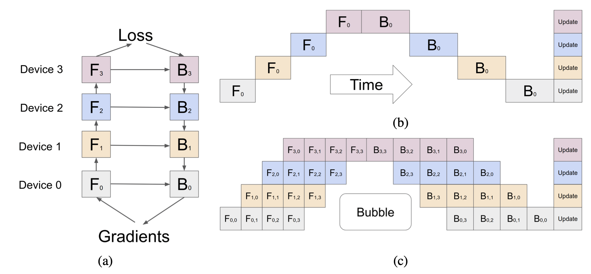
As you can see in part (b) of the diagram, for a pipeline with $N$ devices, each device is active for only $1/N$ of the total time (ignoring communication). This is extremely inefficient and defeats the purpose of using more hardware. The core challenge of making pipeline parallelism effective is to minimize this bubble.

3. Filling the Bubble: Pipelining with Micro-batches

The solution to the bubble problem is conceptually straightforward: instead of processing one large mini-batch at a time, we break it down into several smaller micro-batches.

This allows the first GPU to process the first micro-batch and immediately pass it to the second GPU, while the first GPU begins working on the second micro-batch. This way, we can have multiple micro-batches "in flight" throughout the pipeline at the same time, much like a real assembly line. Part (c) of the "Pipeline Parallelism Bubble" image above illustrates this perfectly.

This technique is the foundation of modern pipeline parallelism implementations like GPipe.

By pipelining micro-batches, we can keep all GPUs busy most of the time, except for a brief "warm-up" phase at the beginning and a "cool-down" phase at the end. This initial and final idle time is the remaining, much smaller, pipeline bubble.

The fraction of time wasted in this bubble is a function of the number of pipeline stages (devices), $n$, and the number of micro-batches, $m$. A simplified formula for the bubble fraction is:

This formula reveals a key trade-off: to minimize the bubble, you need the number of micro-batches ($m$) to be much larger than the number of pipeline stages ($n$). This insight directly influences how you configure your training job.

Conclusion

In this lesson, we have established the fundamental principles of pipeline parallelism, a crucial technique for training extremely deep neural networks.

Key Takeaways:

• Pipeline Parallelism is an inter-layer strategy that partitions a model by assigning consecutive layers to different devices, forming a pipeline.
• It is ideal for deep models where the entire model cannot fit on a single GPU. Its reliance on point-to-point communication makes it more scalable across nodes than tensor parallelism.
• The naive implementation suffers from a massive "pipeline bubble", where only one device is active at a time, leading to poor hardware utilization.
• Modern implementations like GPipe solve this by splitting mini-batches into smaller micro-batches, allowing devices to work concurrently and dramatically reducing the bubble.
• A key design principle is to use a number of micro-batches that is significantly larger than the number of pipeline stages to maximize efficiency.

Preview of the Next Lesson:

We have now introduced the pipeline bubble and its primary mitigation technique, micro-batching. In the next lesson, we will perform a deeper analysis of this bubble overhead. We will explore how different scheduling strategies, such as GPipe's synchronous flush versus PipeDream's 1F1B (one-forward, one-backward) schedule, can further optimize the pipeline by managing memory and reducing idle time. We will also look at advanced techniques like interleaved schedules that rearrange computations to shrink the bubble even more.