Mitigating Bubble Overhead in Pipeline Parallelism

Introduction

In our last lesson, we established that modern pipeline parallelism relies on splitting a training batch into many smaller micro-batches to keep all GPUs in the pipeline busy. We saw that this transforms a massive period of inefficiency—the "pipeline bubble"—into much smaller idle periods at the start ("warm-up") and end ("cool-down") of processing a batch. We approximated the performance impact using the formula: Bubble Fraction $\approx \frac{p-1}{m}$, where $p$ is the number of pipeline stages (devices) and $m$ is the number of micro-batches.

This lesson delves deeper into that bubble. We will move beyond a simple approximation to a more rigorous analysis of this overhead. You will learn how different scheduling strategies can manage the pipeline's execution flow and memory footprint. Most importantly, we will analyze advanced techniques, like interleaved scheduling, that are designed to actively shrink the bubble, and we'll dissect the critical trade-offs these techniques introduce.

By the end of this lesson, you will be able to analyze the factors contributing to pipeline bubble overhead and evaluate the primary methods used to mitigate it.

1. A Formal Look at the Pipeline Bubble

In our previous discussion, the "bubble" represented the collective idle time. Let's formalize this. This idle time occurs because the pipeline must be filled with micro-batches at the beginning of a training step and drained at the end. This process is often called a pipeline flush.

To understand this better, let's watch a short segment that visualizes and quantifies this overhead.

As the video explains, let's define:

• $p$: the number of pipeline stages (i.e., the pipeline depth).
• $m$: the number of micro-batches in a global batch.
• $t_f$: the time to execute the forward pass for one micro-batch on one stage.
• $t_b$: the time to execute the backward pass for one micro-batch on one stage.

At the beginning of a batch, the first micro-batch must traverse all $p$ stages before the last stage can begin its backward pass. This creates an initial ramp-up period. A similar ramp-down occurs at the end. The total time spent in this idle bubble adds up to the time it takes to perform $p-1$ forward passes and $p-1$ backward passes.

• Total Bubble Time: $T_{\text{bubble}}=(p-1)\cdot (t_f+t_b)$
• Ideal Execution Time (if no bubble existed): $T_{\text{ideal}}=m\cdot (t_f+t_b)$

The fraction of time wasted in the bubble is the ratio of these two quantities:

This confirms the simple formula from our last lesson but provides a more rigorous understanding of its origin in the pipeline flush mechanism. This equation makes our primary optimization target clear: to improve efficiency, we must either decrease $p$ or increase $m$.

2. The Impact of Micro-batch Size

The most direct way to reduce the bubble fraction is to increase $m$, the number of micro-batches. Since $m=\frac{\text{Global Batch Size}}{b}$ (where $b$ is the micro-batch size), we can increase $m$ by either increasing the global batch size or decreasing the micro-batch size $b$.

However, this introduces a classic performance trade-off. While a smaller $b$ (and thus larger $m$) reduces the pipeline bubble, it can also decrease single-GPU efficiency. Modern GPUs achieve peak performance on large matrix multiplications. If the micro-batch size is too small, the resulting computations may not be large enough to fully saturate the GPU's computational units, making the workload memory-bound rather than compute-bound.

The paper "Efficient Large-Scale Language Model Training on GPU Clusters" provides a formal analysis of this.

As the paper explains, the total processing time can be modeled as a function of the micro-batch size $b$. A very small $b$ leads to a large $m$, minimizing the $(p-1)/m$ term, but the time per micro-batch, $(t_f(b)+t_b(b))$, increases due to poor GPU utilization. A very large $b$ improves GPU utilization but increases the bubble overhead. This means simply making m as large as possible is not a viable strategy; there's an optimal point to be found.

This limitation motivates the search for other techniques that can reduce the bubble without compromising single-device performance.

3. Advanced Mitigation: Interleaved Schedules

If we can't always increase $m$, perhaps we can reduce the $(p-1)$ term in the bubble fraction. This is the goal of an interleaved pipeline schedule.

The core idea is to break the model into more, smaller partitions (or "chunks") than there are physical devices, and then assign these chunks to devices in an interleaved or round-robin fashion.

Let's say we have a pipeline depth of $p=4$ GPUs. Instead of 4 large model chunks, we could create 8 smaller chunks.

• Standard Schedule: GPU 0 gets layers 1-24, GPU 1 gets 25-48, etc.
• Interleaved Schedule: GPU 0 gets layers 1-12 (chunk 0) AND layers 49-60 (chunk 4). GPU 1 gets layers 13-24 (chunk 1) AND layers 61-72 (chunk 5), and so on.

The image below, taken from the Megatron-LM paper, provides an excellent visualization of how this changes the pipeline's execution flow.

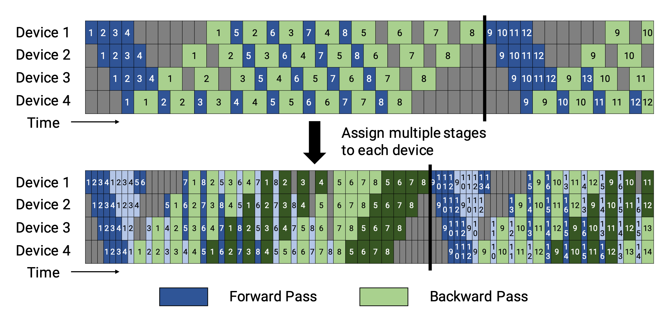
As you can see, the interleaved schedule allows devices to quickly switch to processing a later part of the model (e.g., chunk 4 on device 0) while earlier chunks are still propagating through the pipeline. This leads to a much denser compute schedule and a smaller bubble.

For a deeper dive into the mechanics and trade-offs, let's turn to the paper and a video explanation.

Let's break down the key points from the reading:

1. Bubble Reduction: If we use $v$ interleaved model chunks per device, the time spent in the pipeline flush is reduced by a factor of $v$. The new bubble fraction becomes:

   $$\text{Bubble Time Fraction (Interleaved)}=\frac{1}{v}\cdot \frac{p-1}{m}$$

   This directly attacks the $(p-1)$ component of the overhead, making it highly effective, especially when the number of micro-batches $m$ is small.

2. The Trade-off: Increased Communication: This benefit is not free. In a standard pipeline, GPU i only ever sends data to GPU i+1. In an interleaved schedule, the data flow is more complex. For example, the output of the last chunk on the last device must be sent back to the first device to start the next set of interleaved chunks. The paper notes that the amount of communication also increases by a factor of $v$.

Now, let's watch a final clip that reinforces this concept with experimental results.

The experimental results confirm our theoretical understanding: the interleaved schedule provides a significant throughput boost at small batch sizes where the bubble is the dominant bottleneck. As the batch size (and thus $m$) increases, the original bubble becomes less significant, and the communication overhead of the interleaved schedule starts to offset its benefits, causing the performance gap to close.

Conclusion

In this lesson, we dissected the pipeline bubble, moving from a high-level concept to a quantitative analysis of its causes and mitigation strategies. This provides you with the theoretical grounding to reason about the performance of pipeline-parallel systems.

Key Takeaways:

• The pipeline bubble is the idle time incurred during the "warm-up" and "cool-down" phases of a pipeline flush, and its size relative to useful work is given by the fraction $(p-1)/m$.
• Increasing the number of micro-batches ($m$) is the primary way to amortize bubble overhead, but this is limited by the trade-off between bubble reduction and single-GPU arithmetic intensity (utilization).
• Interleaved schedules offer a more advanced way to mitigate the bubble by partitioning the model into more chunks than devices ($v$), effectively reducing the bubble size by a factor of $v$.
• This benefit comes at a cost: an interleaved schedule also increases the total communication volume by a factor of $v$, creating a critical computation-communication trade-off.
• The optimal strategy depends on the workload: for small batch sizes where the bubble is large, interleaved schedules are highly effective. For large batch sizes, the communication overhead may outweigh the benefits.

Preview of the Next Lesson:

We have now explored data, tensor, and pipeline parallelism in detail. In our next lesson, we will synthesize this knowledge to perform a holistic comparison. We will analyze the different communication patterns (All-Reduce vs. Point-to-Point), memory footprints, and ideal use cases for each paradigm, preparing you to make informed architectural decisions when designing distributed training systems for large-scale models.