Recommended resources
The freely available resources this lesson will direct you to.
Introduction
In our recent lessons, we have explored the three fundamental strategies for distributed training: data parallelism, tensor parallelism, and pipeline parallelism. We've seen how data parallelism replicates a model to process more data simultaneously, how tensor parallelism splits individual layers to fit them into memory, and most recently, how pipeline parallelism divides a model's layers into a sequence of stages to train enormous models, albeit with the challenge of the "pipeline bubble."
This lesson will synthesize these individual concepts into a comprehensive comparative framework. Our goal is to analyze these three paradigms side-by-side, evaluating them on the critical systems-level dimensions that you, as a system designer, care about: their communication patterns, memory consumption, and ideal use cases. Understanding these trade-offs is the key to making informed architectural decisions when designing or optimizing large-scale AI training infrastructure.
By the end of this lesson, you will be able to compare data, tensor, and pipeline parallelism across these dimensions and explain how their strengths and weaknesses guide their use in practice.
A High-Level Comparison
Before we dive into the details, let's start with a visual and tabular overview to frame our discussion. Each parallelism strategy partitions the training problem—model parameters, data, or both—in a distinct way.
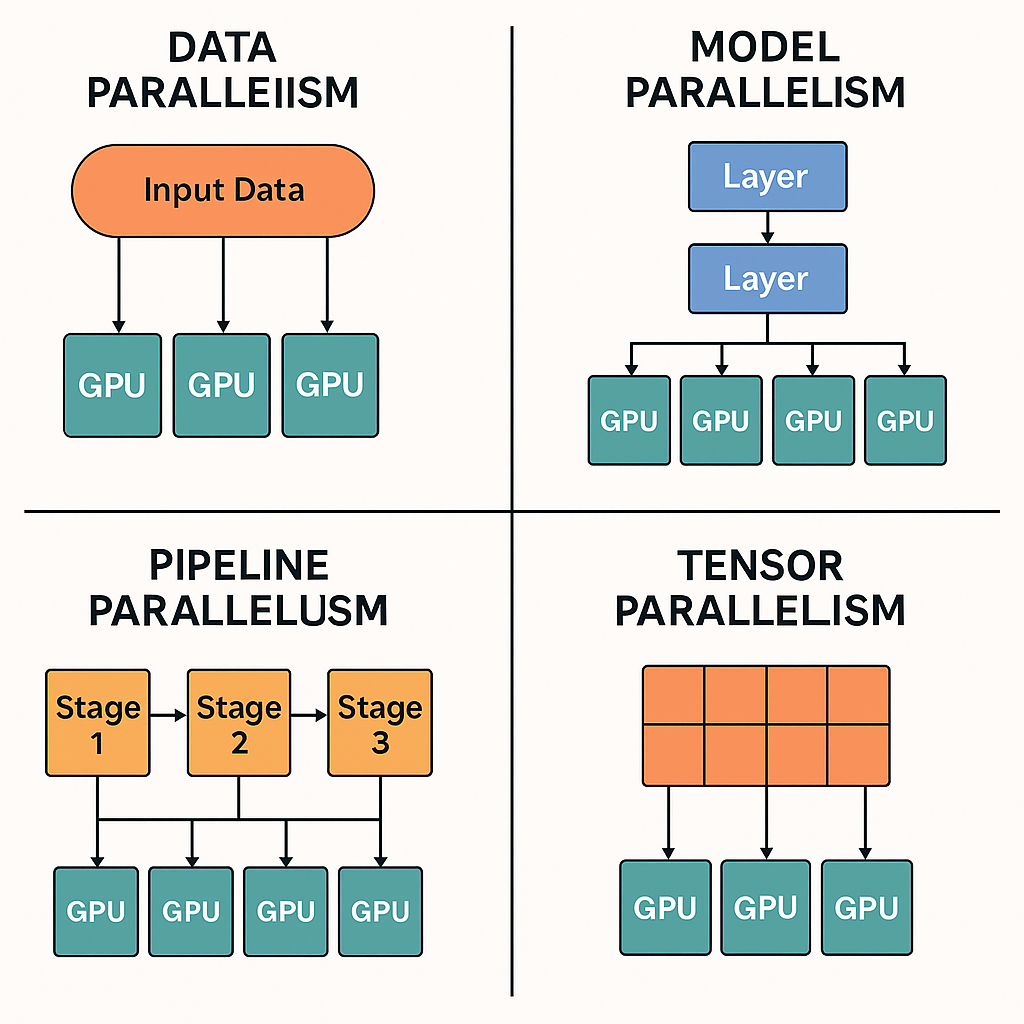
This visual distinction hints at different underlying mechanics. To formalize this, please review the introductory text and comparison table in the following article.
Demystifying Tensor Parallelism
The article 'Demystifying Tensor Parallelism' by Josh Levy-Kramer provides an excellent, concise table that summarizes the pros and cons of each strategy. This will serve as our roadmap for the lesson.
Read the section 'Modes of parallelism', focusing on the descriptions and the summary table. Don't worry about the mathematical details of tensor sharding for now; we will return to those.
The table you've just reviewed highlights three key axes for comparison: communication cost, memory capacity, and implementation complexity/constraints. Let's now explore the first two—communication and memory—in greater detail.
1. Communication Patterns and Costs
The most significant differentiator between these strategies is how, what, and when they communicate. This has profound implications for hardware requirements, particularly the interconnects between GPUs.
For a clear, animated introduction to the communication involved in each paradigm, let's watch a few segments from the following video.
ChatGPT vs Thousands of GPUs! || How ML Models Train at Scale!
The video 'ChatGPT vs Thousands of GPUs!' by Sourish Kundu provides clear, visual explanations of the data flow and synchronization steps for each parallelism type.
Watch the following three clips: Data Parallelism (00:52 - 02:45): Focus on the model replication and the All-Reduce operation used to synchronize gradients. Pipeline Parallelism (05:07 - 06:20): Note how activations are passed from one GPU to the next in a point-to-point fashion. Tensor Parallelism (07:45 - 09:45): Observe how matrix multiplications are split and how All-Gather and All-Reduce primitives are used to combine partial results.
Let's break down the specifics of what you just saw.
Data Parallelism (DP)
- What is communicated: Gradients for the entire model.
- Communication Primitive:
All-Reduce. All GPUs participate in a collective operation to sum gradients and distribute the averaged result back to everyone. - Frequency: Once per training step, after the backward pass and before the optimizer step.
- Cost: The volume of data is proportional to the model size. This can be a significant amount of data, making DP sensitive to the bandwidth of the network fabric.
Pipeline Parallelism (PP)
- What is communicated: Activations (the outputs of a layer).
- Communication Primitive:
Point-to-Point(Send/Receive). GPU i sends its output activations to GPU i+1, which are inputs for the next stage. - Frequency: For every micro-batch, communication occurs between adjacent stages during both the forward and backward passes.
- Cost: The volume of data is proportional to the activation size (
batch_size * sequence_length * hidden_size), not the entire model. This is typically much less data than in DP, making PP less demanding on raw bandwidth and better suited for slower cross-node interconnects. However, it is sensitive to the latency of these point-to-point links.
Tensor Parallelism (TP)
- What is communicated: Partial activations or intermediate results within a layer.
- Communication Primitive:
All-ReduceorAll-Gather, depending on the sharding strategy. - Frequency: Multiple times within a single layer's forward and backward pass.
- Cost: The communication is frequent and tightly coupled with computation. It requires extremely high-bandwidth, low-latency interconnects (like NVLink) to be efficient. Using TP across nodes with slower interconnects like InfiniBand would introduce prohibitive latency.
To understand the communication in TP more deeply, let's refer back to the "Demystifying Tensor Parallelism" article, which explains how the choice of sharding (column-wise vs. row-wise) determines the collective operation used.
Demystifying Tensor Parallelism
This article details how splitting a matrix multiplication requires subsequent communication to ensure the mathematical result is correct.
Please read the sections 'How to shard layers', 'Example: feed-forward transformer layer', and the final 'Summary'. Focus on how a column-wise shard requires an All-Gather and a row-wise shard requires an All-Reduce. Notice how the 'pairwise sharding' pattern cleverly arranges these to eliminate an intermediate communication step.
Summary of Communication
This table summarizes the key distinctions:
| Parallelism | Communication Primitive | What is Communicated | Frequency | Bandwidth Requirement | Best For |
|---|---|---|---|---|---|
| Data | All-Reduce |
Full model gradients | Once per step | High | Scaling throughput |
| Pipeline | Point-to-Point (Send/Recv) |
Activations | Per micro-batch | Low | Cross-node communication |
| Tensor | All-Reduce / All-Gather |
Partial activations | Within each layer op | Very High | Intra-node communication |
2. Memory Usage
The second major difference is how each strategy affects the memory required on each GPU. This determines whether a given model can be trained at all.
-
Data Parallelism: Since the entire model is replicated on every GPU, DP does not reduce the memory footprint. The memory required per GPU is the full size of the model weights, gradients, and optimizer states. This is its primary limitation and the reason model parallelism is necessary for large models.
-
Pipeline & Tensor Parallelism: Both are forms of model parallelism and are designed to solve the memory problem. They do reduce the memory footprint on each device.
- In Pipeline Parallelism, if you split a model across GPUs, each GPU holds roughly of the model's parameters, gradients, and optimizer states.
- In Tensor Parallelism, if you split a layer across GPUs, each GPU holds of that layer's parameters.
- The key benefit is enabling the training of models that are too large to fit in a single GPU's memory.
However, there's a nuance with pipeline parallelism. While it saves on parameter memory, it introduces a new memory cost: storing activations. For the backward pass, each stage must store the input activations for every in-flight micro-batch. If you have a large number of micro-batches () to hide the pipeline bubble, the memory needed to store these activations can become a bottleneck itself.
Summary of Memory Usage
| Parallelism | Model Memory per GPU | Optimizer State Memory per GPU | Enables Larger Models? | Key Memory Consideration |
|---|---|---|---|---|
| Data | Full Model | Full Optimizer States | No | Entire model + optimizer must fit. |
| Pipeline | of Model | of Optimizer States | Yes | Must store activations for all in-flight micro-batches. |
| Tensor | of Model | of Optimizer States | Yes | Reduces memory for weights within a layer. |
3. Ideal Use Cases and Hybrid Strategies
The trade-offs in communication and memory naturally lead to specific use cases for each strategy, which are often combined into powerful hybrid parallelism approaches.
-
Data Parallelism is the simplest and most common. It's the default choice when your model fits on a single GPU and you want to use more GPUs to increase throughput by processing more data in parallel.
-
Pipeline Parallelism is essential when the model is too large for a single GPU. Its low-bandwidth, point-to-point communication makes it the ideal candidate for cross-node parallelism, where communication happens over slower interconnects like InfiniBand or Ethernet.
-
Tensor Parallelism is also used to fit huge models, but its high-bandwidth requirement makes it suitable only for intra-node parallelism, where GPUs are connected by an ultra-fast interconnect like NVLink. It is particularly effective for models with very large layers (e.g., the MLP and attention blocks in Transformers), and it has the advantage of not introducing a "bubble" overhead.
The Rise of 3D Parallelism
Modern systems combine all three in a "3D" arrangement that maps directly onto the physical topology of a GPU cluster:
- Tensor Parallelism is used within a node (e.g., across 8 GPUs connected by NVLink).
- Pipeline Parallelism is used across nodes (e.g., a pipeline stage is a full node of 8 TP-linked GPUs).
- Data Parallelism is used across replicas of the entire pipeline.
This hierarchical approach plays to the strengths of each strategy and the underlying hardware.
Training LLMs at Scale - Deepak Narayanan | Stanford MLSys #83
To see how these trade-offs are navigated in practice, let's watch a segment from the Stanford MLSys seminar by Deepak Narayanan. He quantitatively explores the interaction between tensor and pipeline parallelism.
Watch from 13:45 to 22:58. This is a dense but highly valuable section. Pay close attention to: Why neither tensor nor pipeline parallelism performs well in isolation at large scale. The formula for pipeline bubble size in terms of tensor-parallel size (T) and pipeline-parallel size (P). The graph at 19:22, which shows achieved throughput for different (T, P) configurations. The peak performance at T=8, P=8 is a direct result of balancing the pipeline bubble against the communication cost of tensor parallelism (keeping it within an 8-GPU node).
The analysis in the video provides a concrete example of the architectural reasoning required in system design. The optimal configuration is not a universal constant but emerges from a careful trade-off between the pipeline bubble (minimized by smaller ) and communication overhead (minimized by keeping within a high-speed interconnect domain).
Conclusion
Today, we've dissected and compared the three pillars of distributed training. You now have a framework for analyzing them based on their systems-level characteristics.
Key Takeaways:
- Communication Patterns: Data and Tensor Parallelism rely on bandwidth-heavy collective operations (
All-Reduce,All-Gather), while Pipeline Parallelism uses low-bandwidthPoint-to-Pointcommunication. This makes TP best for intra-node, PP best for cross-node, and DP a flexible but often bandwidth-limited option. - Memory Usage: Data Parallelism offers no memory savings. Both Pipeline and Tensor Parallelism are essential for training models larger than a single GPU's memory by partitioning the model parameters and optimizer states.
- Ideal Use Cases: The choice of strategy is a trade-off. DP maximizes throughput for models that fit in memory. PP and TP overcome memory limits, but PP introduces a pipeline bubble while TP demands expensive, high-speed interconnects.
- Hybrid Strategies: State-of-the-art systems use 3D Parallelism, a hierarchical combination of all three that is carefully mapped to the cluster's network topology to maximize performance.
Preview of the Next Lesson:
We've established why and when you would combine these strategies. In our next lesson, we will delve into the how. We will formally explore hybrid parallelism strategies, like the 3D parallelism used in NVIDIA's Megatron-LM, and analyze how they are implemented in frameworks to train today's largest models.