Data Parallelism: Concepts and Implementation

Introduction

In our last lesson, we conducted a detailed performance analysis of the AllReduce collective operation, comparing Ring and Tree-based algorithms. We established that their efficiency is highly sensitive to message size and the number of nodes, a critical trade-off in distributed systems.

Today, we will zoom out from that specific primitive to understand the broader paradigm where it plays a central role: data parallelism. This lesson directly addresses the learning outcome of describing data parallelism, including how data is partitioned, how gradients are synchronized across devices, and how this is implemented in modern frameworks like PyTorch's DistributedDataParallel (DDP).

This is arguably the most fundamental and widely-used strategy for scaling deep learning training. A thorough grasp of its mechanics, trade-offs, and optimizations is essential for your goal of designing and optimizing large-scale AI systems.

1. The Core Concept of Data Parallelism

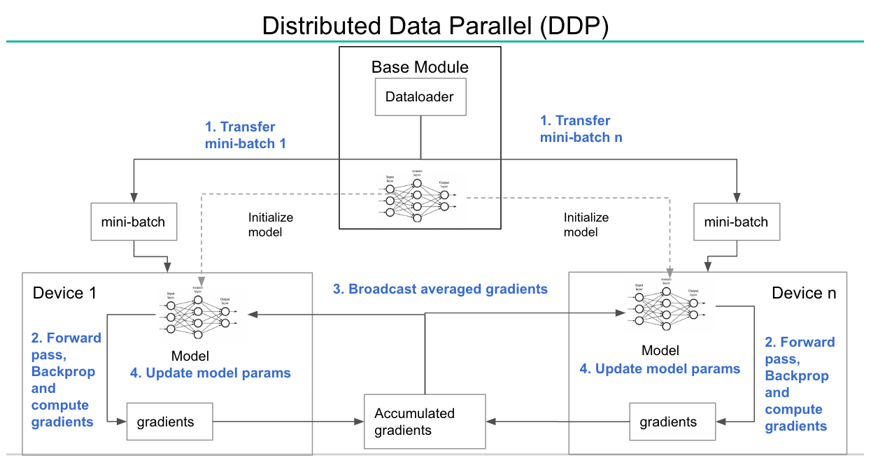
At its heart, data parallelism is an intuitive approach: if one GPU can process a small batch of data, multiple GPUs can process a larger batch in the same amount of time by working in parallel. This involves two main principles:

1. Model Replication: An identical copy of the neural network model is loaded onto each participating GPU (or "worker").
2. Data Partitioning: The global mini-batch of training data is split into smaller "micro-batches," with each worker receiving one micro-batch.

Each worker then performs the forward and backward pass on its own data, computing gradients independently. The crucial step is to ensure that all model replicas stay synchronized. This is achieved by communicating and averaging the gradients from all workers before updating the model weights.

To see this process in action, let's watch a short segment that illustrates the fundamental workflow.

The process described in the video can be summarized by the following diagram:

2. Gradient Synchronization Architectures

The "average gradients" step is the communication-intensive heart of data parallelism. There are two primary architectural patterns for performing this synchronization.

1. Parameter Server (PS): A centralized approach where a set of designated "parameter servers" (often running on CPUs) store the master copy of the model's parameters. Worker GPUs compute gradients and "push" them to the servers. The servers average the gradients, update the parameters, and the workers "pull" the updated parameters back.
2. All-Reduce: A decentralized, peer-to-peer approach where all workers communicate directly with each other to average the gradients. This is typically implemented using a collective operation like AllReduce, which we studied in the previous lesson.

The choice between these two architectures involves significant design trade-offs. For a deeper understanding of these, please read the following text.

As the reading highlights, for training large models on modern GPU clusters with high-speed interconnects (like NVLink), the All-Reduce approach is overwhelmingly preferred. Its ability to utilize inter-GPU bandwidth efficiently without a central bottleneck makes it far more scalable. This is the approach used by PyTorch's DistributedDataParallel.

3. PyTorch DistributedDataParallel (DDP)

Now, let's connect these concepts to a concrete implementation. PyTorch's DistributedDataParallel (DDP) is the canonical framework for data-parallel training. It is designed to be both high-performance and minimally intrusive for the developer.

For your background, understanding the design philosophy of DDP is as important as its mechanics. The following research paper from the PyTorch team explains the core principles.

The paper establishes DDP's core goals: mathematical equivalence to single-node training, high performance, and a simple API. In practice, enabling DDP involves a few key steps:

1. Process Group Initialization: Setting up the communication backend and letting each process know about its peers.
2. Model Wrapping: Encapsulating the nn.Module in a DDP wrapper. This is the "interceptive" API at work; the wrapper handles model replication and gradient synchronization automatically.
3. Data Partitioning: Using a DistributedSampler to ensure each process receives a unique, non-overlapping subset of the data for each epoch.

The following video demonstrates these practical steps.

4. Key Optimizations in Modern Data Parallelism

So far, we've described "naive" data parallelism. However, this approach has two major bottlenecks: one in communication and one in memory. Modern implementations like DDP employ sophisticated techniques to overcome them.

A. Overlapping Communication and Computation

As we know from our previous lesson, AllReduce can be slow. A naive implementation would wait for the entire backward pass to complete before starting a single, large AllReduce operation on all gradients. This leaves the network idle during computation and the compute units idle during communication.

DDP improves this by overlapping communication with computation. It does this by bucketing gradients. As gradients are computed during the backward pass (from the last layer to the first), DDP collects them into buckets. Once a bucket is full, it immediately kicks off an asynchronous AllReduce operation for that bucket's data while the CPU/GPU continues computing gradients for the next layers.

This technique is a perfect example of co-designing algorithms and systems, trading off a small delay (waiting for a bucket to fill) for a large gain in overall throughput by hiding communication latency.

B. Overcoming the Memory Bottleneck: FSDP

The most significant limitation of naive data parallelism is memory. Because every GPU holds a full replica of the model, the memory required for training is not just the model parameters, but also the gradients and the optimizer states (e.g., momentum and variance for Adam).

A key insight from your CS background is that redundant data is a prime target for optimization. The Stanford lecture below brilliantly explains this problem and its modern solution.

The core takeaway is that by sharding the optimizer states, and later the gradients and parameters themselves (in ZeRO stages 2 and 3), FSDP breaks the memory replication constraint of naive data parallelism. Each GPU is only responsible for updating a fraction of the model, dramatically increasing the size of models that can be trained. FSDP is the state-of-the-art implementation of data parallelism within the PyTorch ecosystem and is what you would use for training very large models today.

Conclusion

In this lesson, we've built a comprehensive understanding of data parallelism, from its simple core concept to the sophisticated optimizations used in modern frameworks.

Key Takeaways:

• Data Parallelism is a training paradigm based on model replication and data partitioning.
• Gradient synchronization is the key communication step, and the decentralized All-Reduce architecture is dominant for high-performance GPU training.
• PyTorch DDP provides a non-intrusive API that automates this process by wrapping the model and using a DistributedSampler.
• Naive data parallelism suffers from two main bottlenecks:
  1. Communication Overhead: Mitigated by gradient bucketing and overlapping communication with computation.
  2. Memory Redundancy: Mitigated by sharding the optimizer states, gradients, and parameters, as implemented in PyTorch FSDP (based on ZeRO).

Preview of the Next Lesson:

Data parallelism is incredibly powerful for scaling throughput, and with FSDP, it can also accommodate very large models. However, there are scenarios where the model's layers themselves are so large that a single layer's activations or parameters cannot fit onto one GPU. In these cases, we must turn to model parallelism. In our next lesson, we will explore the first type: tensor parallelism, which partitions individual model layers across multiple GPUs.