Critical Slowing Down: From Observation to Origin

Recommended resources

The freely available resources this lesson will direct you to.

Lecture 8 Ising model From enumeration to Cluster Monte Carlo Simulations École normale supériewww.youtube.com
[PDF] Chapter 3 Monte Carlo Simulations in Statistical Physicswww.physik.uni-leipzig.de
[PDF] arXiv:1404.0209v1 [cond-mat.stat-mech] 1 Apr 2014arxiv.org

Hello! Welcome back to our exploration of computational methods.

In the previous lesson, we built the foundational tool for our computational laboratory: the Metropolis Monte Carlo algorithm for the 2D Ising model. You now have a working simulation that can generate configurations according to the Boltzmann distribution at any given temperature.

Today, we will put that simulation to the test in the most interesting regime: near the critical point. Our learning outcome is to observe critical slowing down in simulations and explain its origin from the diverging correlation time. We will see that as we approach the critical temperature $T_{c}$ , our simple local-update algorithm becomes dramatically inefficient. This is not just a computational quirk; it is a direct and observable manifestation of the critical phenomena we have studied theoretically, namely the divergence of the correlation length.

1. From Correlated Steps to Correlated Time

A key feature of a Markov Chain Monte Carlo simulation is that the generated configurations are not statistically independent. Each state is a small modification of the one before it. This introduces a "memory" or temporal correlation into our data. To perform a proper statistical analysis, we must understand how long it takes for the system to "forget" its past state.

This is quantified by the autocorrelation function. For an observable like the total magnetization $M$ , its autocorrelation function is defined as:

A_{M} (t) = \frac{⟨ M ( t _{0} ) M ( t _{0} + t )⟩ - ⟨ M ⟩ ^{2}}{⟨ M ^{2} ⟩ - ⟨ M ⟩ ^{2}}

Here, $t$ represents the "time" separation in units of Monte Carlo sweeps. This function measures how correlated the magnetization is with itself after $t$ sweeps. Typically, for large $t$ , this function decays exponentially:

A_{M} (t) \sim e^{- t / τ_{M}}

This decay constant, $τ_{M}$ , is the exponential autocorrelation time. It represents the characteristic time, in sweeps, required for the system's magnetization to become decorrelated from its initial value.

To get a more formal handle on this concept and its implications, please read the following section from the lecture notes by W. Janke.

Chapter 3 Monte Carlo Simulations in Statistical Physics by W. Janke

These notes provide a clear, quantitative introduction to temporal correlations in Monte Carlo simulations.

Please read Section 2.4, 'Temporal correlations' (pages 105-106). Focus on the definition of the autocorrelation function (Eq. 23) and the exponential autocorrelation time (Eq. 24). The figures and discussion for the 2D Ising model provide a concrete example.

2. Observing Critical Slowing Down

Now, let's use your simulation to see what happens to this autocorrelation time as we approach the critical temperature of the 2D Ising model, $T_{c} = \frac{2 J}{k _{B} l n ( 1 + 2 )} \approx 2.269 J / k_{B}$ .

If you were to plot the magnetization versus Monte Carlo time (sweeps) for different temperatures, you would observe three distinct behaviors:

High Temperature ( $T ≫ T_{c}$ ): The system is in the paramagnetic phase. Thermal fluctuations are strong, and spins are weakly correlated. The magnetization fluctuates rapidly and symmetrically around zero. The autocorrelation time $τ$ is very short.
Low Temperature ( $T ≪ T_{c}$ ): The system is in the ferromagnetic phase. The magnetization stays close to its spontaneous value ( $+ M_{s a t}$ or $- M_{s a t}$ ) and fluctuates with small, rapid oscillations around it. The autocorrelation time for these small fluctuations is also short.
Critical Temperature ( $T \approx T_{c}$ ): The behavior changes dramatically. The magnetization undertakes slow, large-scale wanderings that span a wide range of values. The system seems "indecisive," forming large correlated domains that take a very long time to evolve or disappear.

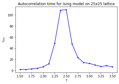
This dramatic increase in the autocorrelation time near the critical point is the phenomenon of critical slowing down.

The following plot shows the results of a systematic study of the autocorrelation time as a function of temperature.

Autocorrelation Time for 2D Ising Model — Plot of the autocorrelation time $\tau$ versus temperature $T$ for an Ising model simulation. The sharp peak demonstrates that the time needed for the system to generate a statistically independent configuration diverges as the temperature approaches its critical value $T_c \approx 2.27$.

Test your understanding!

Based on the physics of the ordered and disordered phases, what is the fundamental difference in the long-time behavior of the magnetization time-series at $T ≪ T_{c}$ versus $T ≫ T_{c}$ ? (Ignore the initial equilibration phase).

Show answer

At $T ≫ T_{c}$ (paramagnetic phase), the average magnetization $⟨ M ⟩$ is zero. The time-series will show fluctuations that are symmetric around $M = 0$ .

At $T ≪ T_{c}$ (ferromagnetic phase), spontaneous symmetry breaking occurs. The system will pick one of the two ground states, with magnetization $⟨ M ⟩ \approx + M_{s a t}$ or $⟨ M ⟩ \approx - M_{s a t}$ . The time-series will show fluctuations around one of these non-zero values. For a finite simulation time on a large lattice, it's very unlikely to see the system flip between the $+ M_{s a t}$ and $- M_{s a t}$ states.

3. The Physical Origin: From Correlation Length to Correlation Time

Critical slowing down is a direct consequence of the physics of critical phenomena we've already studied. The key is to connect the temporal correlation $τ$ to the spatial correlation length $ξ$ .

Let's review the physical picture and then formalize it.

Lecture 8 Ising model From enumeration to Cluster Monte Carlo Simulations École normale supérie

This video section gives a concise qualitative explanation for why local Monte Carlo algorithms suffer from critical slowing down.

Watch the segment from 10:52 to 11:54. The speaker explains how the increase in correlation length near T_c makes it difficult for local updates to change large correlated regions.

As the video explains, the core of the problem lies in the mismatch between the algorithm's actions and the system's state:

System's State near $T_{c}$ : The correlation length $ξ$ diverges. This means spins form large, correlated domains that can span a significant fraction of the system size. The system is characterized by fluctuations on all length scales up to $ξ$ .
Algorithm's Action: The Metropolis algorithm performs local updates. It flips one spin at a time.

To change the overall magnetization, the algorithm needs to flip a large number of spins inside a correlated domain. However, flipping a single spin deep inside a domain of aligned neighbors is energetically very costly and thus has an exponentially small acceptance probability. The only effective way for a local algorithm to alter these large domains is by slowly "eroding" them from the edges. This process is analogous to diffusion and is extremely slow.

This relationship is formalized through the introduction of a new exponent, the dynamic critical exponent $z$ . It connects the correlation time to the correlation length via a power law:

τ \propto ξ^{z}

Since we know $ξ \propto ∣ T - T_{c} ∣^{- ν}$ , the autocorrelation time diverges as we approach the critical point:

τ \propto ∣ T - T_{c} ∣^{- ν z}

In a finite system of linear size $L$ simulated exactly at $T_{c}$ , the correlation length is capped by the system size, $ξ \sim L$ . This leads to a power-law scaling of the autocorrelation time with the system size itself:

τ \propto L^{z}

For local algorithms like Metropolis applied to the Ising model, the dynamic exponent is found to be $z \approx 2.17$ . This means that doubling the system size increases the required simulation time by more than a factor of four to get the same number of independent samples.

The following resources provide more depth on this crucial connection.

An introduction to Monte Carlo methods by Walter and Barkema

This paper by Walter and Barkema provides an excellent physical argument for critical slowing down and the scaling of the correlation time.

Please read Section 4, 'Cluster algorithms' (pages 6-8) and Section 7, 'Dynamical aspects' (pages 12-15). Section 4 gives a very clear motivation for why local algorithms fail near T_c. Section 7 provides a detailed discussion of correlation time and its scaling behavior, including the definition of the dynamic critical exponent z (see Eq. 16 and 19).

4. Consequences and the Path Forward

Critical slowing down is not just a theoretical curiosity; it has severe practical consequences for simulations.

Long Equilibration Times: The time required to reach thermal equilibrium, $τ_{e q}$ , is proportional to the autocorrelation time $τ$ . Near $T_{c}$ , you must run your simulation for an extremely long time before you can even begin taking measurements.
High Statistical Errors: The statistical error of an observable's mean value depends on the number of independent samples, $N_{e ff}$ . This effective sample size is related to the total number of measurements $N$ and the autocorrelation time by $N_{e ff} = N / (2 τ_{in t})$ , where $τ_{in t}$ is the closely related integrated autocorrelation time. As $τ$ diverges, $N_{e ff}$ plummets, and achieving acceptable precision requires prohibitively long simulation runs. The Janke paper (LINK) discusses this in detail in Section 3.1.3.

The fundamental problem is the local nature of the Metropolis algorithm. The solution, therefore, must involve non-local updates. This is the motivation for cluster algorithms, such as the Swendsen-Wang or Wolff algorithms. These methods intelligently identify a correlated cluster of spins and flip them all at once. By changing the system on a scale comparable to the correlation length, they can dramatically reduce the dynamic critical exponent $z$ .

Comparison of Critical Slowing Down in 2D Ising Model Simulations — A log-log plot comparing the scaling of autocorrelation time $\tau$ with system size $L$ for the local Metropolis algorithm versus the non-local Swendsen-Wang cluster algorithm. The much smaller dynamic exponent $z$ for the cluster algorithm demonstrates its massive efficiency advantage in mitigating critical slowing down.

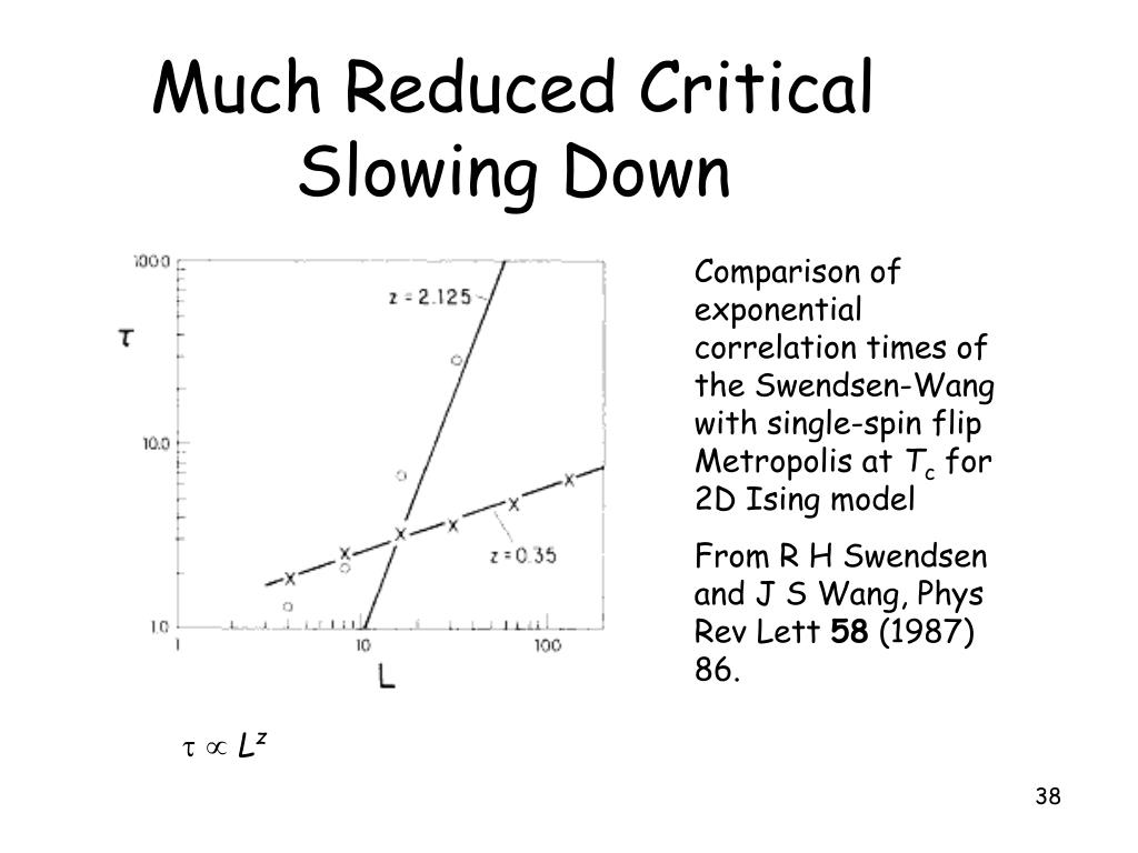
As this plot shows, cluster algorithms don't eliminate critical slowing down, but they reduce it so effectively that they become the essential tool for high-precision studies of critical phenomena.

Conclusion

In this lesson, we have encountered a crucial practical barrier in the computational study of phase transitions and connected it directly to the underlying physics.

Key Takeaways:

Monte Carlo simulations generate temporally correlated configurations, characterized by an autocorrelation time $τ$ .
Near a critical point, local update algorithms exhibit critical slowing down, where $τ$ diverges.
This phenomenon is a direct result of the diverging spatial correlation length $ξ$ . Local updates are inefficient at altering large, correlated domains.
The relationship is formalized by the dynamic critical exponent $z$ , through the scaling relations $τ \propto ξ^{z}$ and $τ \propto L^{z}$ .
Critical slowing down poses a major practical problem, leading to long equilibration times and large statistical errors.

Preview of the Next Lesson:

Having diagnosed the problem, we will now turn to the solution. In the next lesson, we will focus on the learning outcome: "Describe a cluster algorithm (e.g., Wolff) and explain how it mitigates critical slowing down." We will see how this elegant algorithm works and why it is so much more powerful than the local methods we have used so far.