Wolff Algorithm and Critical Slowing Down

Hello! Welcome to the next lesson in our computational module.

In our last session, we confronted a major challenge in simulating systems near a critical point: critical slowing down. We saw that as the correlation length $\xi$ diverges, local update algorithms like Metropolis become extraordinarily inefficient, with the autocorrelation time $\tau$ scaling as $\tau \propto L^z$, where the dynamic exponent $z$ is large. This happens because single-spin flips are fundamentally mismatched to the large-scale correlated domains that dominate the physics at criticality.

Today, we'll explore the solution. Our learning outcome is to describe a cluster algorithm (e.g., Wolff) and explain how it mitigates critical slowing down. We will dissect an elegant and powerful algorithm that performs non-local updates, designing its moves to match the correlation structure of the system itself. This approach dramatically reduces the dynamic exponent $z$, making high-precision simulations of critical phenomena feasible.

1. The Core Idea: From Local Flips to Cluster Flips

The failure of local updates points directly to the solution: we need an algorithm that can perform collective, non-local moves. The first major breakthrough in this direction was the Swendsen-Wang (SW) algorithm. While we will focus on its successor, the Wolff algorithm, understanding the SW approach provides valuable context for the key conceptual leap.

The SW algorithm is based on a deep connection between the Ising model and the random cluster model, established by Fortuin and Kasteleyn. It allows one to map the spin configuration onto a graph problem.

In essence, the SW algorithm proceeds as follows:

1. Bond Formation: Go through every pair of nearest-neighbor spins on the lattice. If they are aligned (e.g., both are spin-up), "freeze" a bond between them with probability $p=1-e^{-2\beta J}$.
2. Cluster Identification: Identify all the connected clusters of spins based on these new bonds. The entire lattice is now partitioned into disjoint clusters.
3. Cluster Flipping: For each cluster, decide with 50% probability whether to flip all the spins within it or leave them as they are.

The SW algorithm was revolutionary because it flips entire correlated domains at once, drastically improving performance near $T_c$. However, it still spends considerable computational effort identifying and processing all clusters, many of which might be very small and inconsequential. This observation led to a more efficient, targeted variant.

2. The Wolff Algorithm: A Single-Cluster Approach

The Wolff algorithm refines the SW idea by focusing the computational effort where it matters most: on a single, potentially large, cluster. Instead of partitioning the whole lattice, it grows one cluster from a random starting point and always flips it.

The procedure is elegant and, given your experience with simulations, you'll recognize that it can be implemented efficiently using a stack or queue (akin to a depth-first or breadth-first search).

Let's formalize the steps for the ferromagnetic Ising model:

1. Seed Selection: Choose a single lattice site $i$ uniformly at random. Note its spin value, $\sigma =s_i$.
2. Cluster Growth: Create a "to-do" list (e.g., a stack) and add the seed site $i$ to it. The cluster $C$ initially contains only $i$.
3. Iterate: While the to-do list is not empty:
   a. Pop a site $j$ from the list.
   b. Consider each nearest neighbor $k$ of site $j$.
   c. If site $k$ has the same spin as the original seed ($s_k=\sigma$) and is not yet in the cluster $C$, add it to the cluster $C$ with probability $p_{\text{add}}=1-e^{-2\beta J}$.
   d. If you decide to add site $k$, also push it onto the to-do list.
4. Flip: Once the to-do list is empty, the cluster growth is complete. Flip the sign of every spin within the final cluster $C$: for all $j\in C$, set $s_j\to -s_j$.

This entire process constitutes a single Wolff move. Note that it is rejection-free; the proposed move is always accepted.

3. Why It Works: The Detailed Balance Condition

For any MCMC algorithm to be valid, it must generate states according to the desired probability distribution (the Boltzmann distribution, $\pi (s)\propto e^{-\beta H(s)}$). A sufficient condition for this is satisfying detailed balance:

where $P(s\to s^{\prime })$ is the transition probability from state $s$ to $s^{\prime }$.

The specific choice of $p_{\text{add}}=1-e^{-2\beta J}$ is not arbitrary; it is precisely what's needed to satisfy detailed balance. The proof is a beautiful piece of statistical physics reasoning.

Let's summarize the key steps of the proof:

• The transition $s\to s^{\prime }$ is defined by flipping a specific cluster $C$. The reverse move, $s^{\prime }\to s$, involves flipping the exact same cluster $C$.
• The probability of generating the cluster $C$ in state $s$ depends on the bonds that were not formed at its boundary. Let the boundary of $C$ have $m$ edges connecting it to external spins of the same sign, and $n$ edges connecting it to external spins of the opposite sign. The probability of forming exactly $C$ (and no larger) is proportional to $(1-p_{\text{add}}{)}^m$, as each of the $m$ potential growth steps was rejected.
• In the flipped state $s^{\prime }$, the roles are reversed. The same boundary now has $n$ edges connecting to external spins of the same sign and $m$ to spins of the opposite. The probability of forming $C$ to flip it back is proportional to $(1-p_{\text{add}}{)}^n$.
• The ratio of forward to backward transition probabilities is therefore $\frac{P(s\to s^{\prime })}{P(s^{\prime }\to s)}\propto (1-p_{\text{add}}{)}^{m-n}$.
• The energy change also depends only on the boundary. The change in energy upon flipping $C$ is $\Delta H=H(s^{\prime })-H(s)=2J(m-n)$.
• The ratio of Boltzmann factors is $\frac{\pi (s^{\prime })}{\pi (s)}=e^{-\beta \Delta H}=e^{-2\beta J(m-n)}$.
• Detailed balance requires $\frac{P(s\to s^{\prime })}{P(s^{\prime }\to s)}=\frac{\pi (s^{\prime })}{\pi (s)}$. Plugging in our results gives: $$(1-p_{\text{add}}{)}^{m-n}=(e^{-2\beta J}{)}^{m-n}$$ This holds if and only if $p_{\text{add}}=1-e^{-2\beta J}$, which is exactly the probability we use.

4. How Wolff Mitigates Critical Slowing Down

The brilliance of the Wolff algorithm is that the size and shape of its updates are not fixed, but adapt to the physical state of the system.

• High Temperatures ($T\gg T_c$): $\beta$ is small, so $p_{\text{add}}\approx 2\beta J$ is also small. The cluster rarely grows beyond the initial seed spin. The algorithm behaves like a single-spin flip, which is efficient in the disordered phase where correlations are short-ranged.
• Low Temperatures ($T\ll T_c$): $\beta$ is large, so $p_{\text{add}}\to 1$. The cluster will grow to encompass almost the entire system (assuming it's well-ordered). The algorithm flips huge chunks of the system, allowing it to tunnel between the $+M$ and $-M$ ground states far more effectively than Metropolis.
• Near Criticality ($T\approx T_c$): This is where the magic happens. The correlation length $\xi$ is large, and the system exhibits correlated domains on all length scales up to $\xi$. The Wolff algorithm, by its very construction, also builds clusters whose typical size scales with $\xi$. It naturally generates moves on the same scale as the system's correlations, allowing it to efficiently update the large-scale structures that cause critical slowing down in local algorithms.

This dramatic effect is best visualized by comparing the scaling of the autocorrelation time $\tau$ with system size $L$.

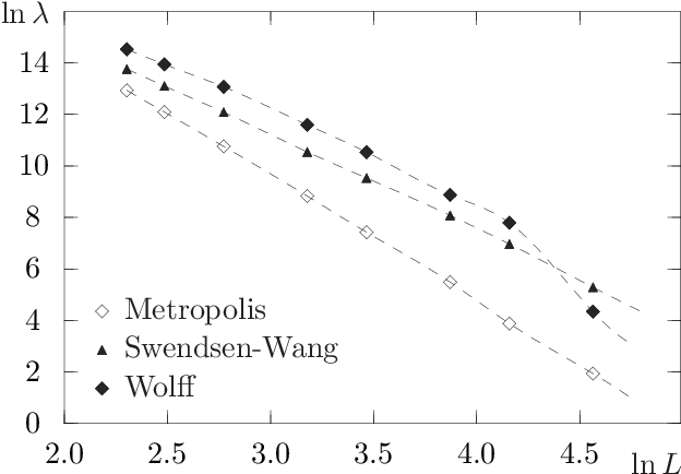
The plot shows that the dynamic exponent $z$ for Wolff is close to zero, while for Metropolis it's over 2. This difference is staggering. To simulate a system 10 times larger, Metropolis requires over $10^2=100$ times the computational effort to get one independent sample, whereas Wolff requires only $10^{0.3}\approx 2$ times the effort.

Conclusion

Today we have moved from diagnosing a problem to implementing a powerful solution. Cluster algorithms represent a major milestone in computational statistical physics.

Key Takeaways:

• Cluster algorithms overcome critical slowing down by performing non-local updates.
• The Wolff algorithm is an efficient single-cluster method that grows a cluster from a random seed by adding aligned neighbors with probability $p_{\text{add}}=1-e^{-2\beta J}$ and then flips the entire cluster.
• This specific choice of $p_{\text{add}}$ ensures the algorithm satisfies detailed balance and correctly samples the Boltzmann distribution.
• The algorithm's power lies in its adaptive nature: the size of the update (the cluster) naturally scales with the system's correlation length, directly countering the source of critical slowing down and dramatically reducing the dynamic exponent $z$.

Preview of the Next Lesson:

Now that we have a tool to efficiently generate high-quality, decorrelated configurations near $T_c$, our next step is to learn how to extract the maximum amount of information from a single simulation run. In the next lesson, we will cover the learning outcome: "Apply the histogram reweighting technique to extrapolate simulation results to nearby temperatures from a single run." This powerful analysis method allows us to map out the behavior of thermodynamic quantities over a range of temperatures using data from just one simulation, making our studies even more efficient.