Simulating the 2D Ising Model with Metropolis Monte Carlo

Hello! Welcome to the first lesson in our module on computational methods.

Over the past eleven modules, we have built a substantial theoretical edifice for understanding phase transitions and critical phenomena. We've journeyed from classical thermodynamics through mean-field and Landau theories, all the way to the powerful but abstract frameworks of the renormalization group and scaling hypotheses. You've seen how these theories predict universal behaviors, described by critical exponents and scaling functions.

Today, we pivot from pure theory to computation. Our goal is to develop the primary tool used to test these theories, explore models without exact solutions (like the 3D Ising model), and gain a concrete, dynamic intuition for the phenomena we've been studying.

This lesson's learning outcome is to implement the Metropolis Monte Carlo algorithm to simulate the 2D Ising model. We will break down the "why" and the "how" of this foundational algorithm, which enables us to generate representative configurations of a system in thermal equilibrium. This will be a practical lesson that leverages your programming skills, providing a computational laboratory for the physics we've learned.

A quick note connecting to our previous topic: in the last module, we discussed dynamic critical phenomena, particularly "critical slowing down." The simple algorithm we will implement today is famously susceptible to this issue. While our focus today is just on getting the simulation working correctly, in the next lesson, we will see this slowing down in action and understand why more advanced algorithms are needed near a critical point.

1. The Challenge of Statistical Averages and the Idea of Importance Sampling

Recall that for a system described by a Hamiltonian $H$, the thermal average of an observable $O$ is given by:

where the sum is over all possible configurations $C$ of the system, $E(C)$ is the energy of a configuration, $\beta =1/(k_{B}T)$, and $Z$ is the partition function.

The fundamental computational challenge is the size of this sum. For an $L\times L$ Ising model, there are $N=L^2$ spins, leading to $2^N$ configurations. As noted in the paper by Walter and Barkema (LINK), even for a tiny $10\times 10\times 10$ 3D system, this is $\sim 10^{301}$ states—a number far beyond any possibility of direct enumeration.

The solution is not to sample every state, but to sample the important ones. The Boltzmann factor $e^{-\beta E(C)}$ tells us that at any given temperature, configurations with low energy contribute exponentially more to the average than those with high energy. This leads to the strategy of importance sampling: we want to generate a sequence of configurations in such a way that the probability of a configuration appearing in our sequence is proportional to its Boltzmann weight.

2. Markov Chain Monte Carlo

A powerful method for achieving importance sampling is Markov Chain Monte Carlo (MCMC). The core idea is to construct a "random walk" through the space of all possible configurations. This walk is a Markov chain, meaning the next step in the walk only depends on the current configuration, not the history of how we got there.

To ensure this random walk correctly samples the Boltzmann distribution, the process must satisfy two key properties.

As the paper explains, the two crucial conditions are:

1. Ergodicity: It must be possible to get from any configuration with a non-zero Boltzmann weight to any other such configuration in a finite number of steps. For our Ising model, where a "step" will involve flipping a single spin, this condition is met. You can transform any configuration into any other by flipping spins one by one.

2. Detailed Balance: A sufficient (though not strictly necessary) condition for ensuring the chain converges to the correct equilibrium distribution $P(C)\propto e^{-\beta E(C)}$ is detailed balance. For any two configurations $A$ and $B$, the rate of transitions from $A$ to $B$ must equal the rate of transitions from $B$ to $A$ in equilibrium:

   $$P_{eq}(A)W(A\to B)=P_{eq}(B)W(B\to A)$$

   Here, $W(A\to B)$ is the transition probability of moving from state $A$ to $B$. Since $P_{eq}(A)/P_{eq}(B)=e^{-\beta (E_A-E_B)}$, our task is to design transition probabilities $W$ that satisfy this condition.

3. The Metropolis Algorithm

The Metropolis algorithm (or more generally, Metropolis-Hastings) is a brilliant and simple recipe for constructing transition probabilities $W$ that satisfy detailed balance. The transition $W(A\to B)$ is broken into two sub-steps:

• Proposal: Propose a move from $A$ to a new trial configuration $B$ with probability $T(A\to B)$.
• Acceptance: Accept this proposed move with probability $A(A\to B)$.

Thus, $W(A\to B)=T(A\to B)\times A(A\to B)$.

For the Ising model, the simplest approach is to use a symmetric proposal:

1. Proposal: Select a single spin at random from the $N$ spins on the lattice and propose to flip it.
2. The trial configuration $B$ is the same as $A$, but with one spin flipped. The probability of proposing this specific move is $1/N$. The probability of proposing the reverse move (starting in $B$ and flipping the same spin to get back to $A$) is also $1/N$. So, $T(A\to B)=T(B\to A)$.

With a symmetric proposal, the detailed balance condition simplifies considerably:

The genius of the Metropolis algorithm is its choice for the acceptance probability, which satisfies this ratio while maximizing the acceptance rate:

This rule has a clear physical interpretation:

• If flipping the spin lowers the energy ($\Delta E\le 0$), the move is always accepted ($A=1$). This drives the system towards lower energy states.
• If flipping the spin increases the energy ($\Delta E>0$), the move is accepted with a probability $e^{-\beta \Delta E}<1$. This is the crucial step that allows the system to escape from local energy minima and explore the full configuration space, simulating the effect of thermal fluctuations.

The following resource provides a very clear step-by-step guide to implementing this logic.

4. Implementation Details for the 2D Ising Model

Let's consolidate the information from the resources into a concrete plan for implementation. Your background in Python and C++ will make this straightforward.

The Algorithm Flow

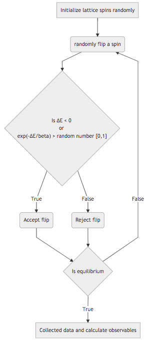
The overall process follows a simple loop, which is nicely visualized in this flowchart:

Key Implementation Steps

1. System Representation: An $L\times L$ array (e.g., a NumPy array in Python) is perfect for storing the spin configuration, with values $\pm 1$. Remember to handle periodic boundary conditions. For a spin at site $(i,j)$, its neighbors are at $((i\pm 1)\%L,j)$ and $(i,(j\pm 1)\%L)$, where % is the modulo operator.

2. Efficient $\Delta E$ Calculation: As highlighted in the Illinois resource, you should not recalculate the total energy of the system after every flip. This would be an $O(L^2)$ operation. The change in energy only depends on the spin being flipped and its immediate neighbors. The Ising Hamiltonian is $H=-J{\sum }_{⟨ij⟩}{s}_i{s}_j$. The local energy contribution involving a spin $s_k$ is $E_k=-J{s}_k{\sum }_{i\in \text{nn}(k)}{s}_i$. If you flip $s_k\to -s_k$, the new local energy is $E_k^{\prime }=-J(-s_k){\sum }_{i\in \text{nn}(k)}{s}_i=-E_k$. The change in total energy is thus:

   $$\Delta E=E_k^{\prime }-E_k=-2E_k=2J{s}_k\sum _{i\in \text{nn}(k)}{s}_i$$

   This is an $O(1)$ calculation, as it only involves a fixed number of neighbors (4 for a 2D square lattice).

3. The Monte Carlo Step: A function that performs one step of the algorithm would look like this:

   • Choose a random lattice site $(i,j)$.
   • Calculate $\Delta E$ for flipping the spin $s_{i,j}$ using the formula above.
   • Generate a uniform random number r between 0 and 1.
   • If r < exp(-β * ΔE), flip the spin: spins[i,j] *= -1. This single condition works for both positive and negative $\Delta E$, since exp(-β * ΔE) will be greater than 1 if $\Delta E$ is negative.

4. Sweeps, Equilibration, and Measurement:

   • Sweep: The natural unit of "time" in the simulation is one Monte Carlo sweep, which consists of $N=L^2$ attempted spin flips.
   • Equilibration: When you start a simulation (e.g., from a random or fully ordered state), the system is not in equilibrium. You must run the simulation for a certain number of "equilibration sweeps" to let it relax. You can monitor a macroscopic quantity like the total energy or magnetization to see when it has stabilized around an average value.
   • Measurement: After equilibration, you can begin collecting data. For example, after each sweep, you can calculate and record the total energy $E$ and total magnetization $M=\sum s_i$. After many measurement sweeps, you can average these recorded values to find $⟨E⟩$ and $⟨M⟩$.

Conclusion

In this lesson, we have laid the groundwork for simulating statistical systems. You now have the complete conceptual and algorithmic recipe to implement the Metropolis Monte Carlo simulation for the 2D Ising model.

Key Takeaways:

• Direct enumeration of states is computationally impossible for non-trivial systems.
• Importance sampling is a strategy to preferentially sample configurations with high Boltzmann weights.
• Markov Chain Monte Carlo (MCMC) methods, like the Metropolis algorithm, generate a sequence of states that accomplishes this.
• The algorithm's validity rests on the principles of ergodicity and detailed balance.
• The Metropolis algorithm uses a simple but powerful acceptance rule, $A=\min (1,e^{-\beta \Delta E})$, which allows the system to find thermal equilibrium.
• For the Ising model, an efficient implementation requires an O(1) calculation of the local energy change $\Delta E$.

Preview of the Next Lesson:

Now that you have the tools to build the simulation, the next step is to analyze its behavior. As we approach the critical temperature $T_c$, you will find that the simulation takes longer and longer to equilibrate and for successive configurations to become statistically independent. This is critical slowing down—the direct computational consequence of the diverging correlation length and time we discussed theoretically. In the next lesson, we will observe this phenomenon in our simulation and quantify it, which will motivate the need for more advanced cluster algorithms.