Vortex-Antivortex Unbinding and the Kosterlitz-Thouless Transition

Recommended resources

The freely available resources this lesson will direct you to.

Hello! Welcome to the next lesson in our study of advanced topics in critical phenomena.

In our previous session, we introduced the Kosterlitz-Thouless (KT) transition in the 2D XY model. We established that this unique phase transition is driven not by the ordering of spins, but by the behavior of topological defects called vortices. We saw that at low temperatures, vortices exist as bound vortex-antivortex pairs, preserving a "quasi-long-range" order. At high temperatures, these pairs unbind, creating a disordered plasma of free vortices.

The key question we ended with was: how does this unbinding happen? It's a collective effect, where the presence of many pairs influences the fate of any single pair. Today, our goal is to dive into the beautiful physics of this mechanism. We will explain the role of vortex-antivortex pair unbinding in driving the KT transition by using a powerful analogy and the framework of the renormalization group.

1. The Big Picture: Screening and Unbinding

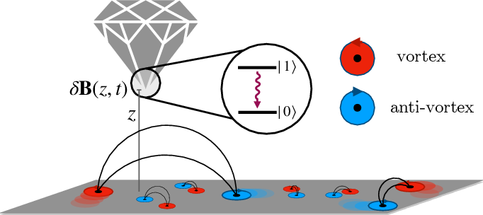
At its heart, the unbinding transition is an elegant example of screening. In the low-temperature phase, the system is a dilute "gas" of bound vortex-antivortex pairs. As the temperature rises, more of these pairs are created by thermal fluctuations. These pairs, being composed of opposite "charges," act like tiny, neutral dipoles.

A large, loosely-bound pair finds itself in a sea of smaller, transient pairs. This sea of dipoles acts like a dielectric medium, screening the logarithmic attraction that holds the large pair together. As the temperature increases, the density of these screening pairs rises, weakening the effective force until, at $T_{K T}$ , the binding force over long distances vanishes. The pair unbinds, and free vortices proliferate.

Vortex-Antivortex Pairs and Quantum Sensing — A visual representation of the system. Vortices (red) and anti-vortices (blue) populate the 2D plane. At low temperatures, they form tightly bound pairs (connected by black arcs). The KT transition is driven by the unbinding of these pairs into free charges, a process we can analyze with the tools of statistical mechanics.

To make this intuitive picture precise, we first need to formalize the analogy between a system of vortices and a system of interacting charges.

2. From Spins to Charges: The 2D Coulomb Gas

The genius of the KT analysis lies in shifting focus from the underlying spin field $θ (r)$ to the vortices themselves. By cleverly manipulating the XY model Hamiltonian, one can show that the part of the energy associated with a static configuration of vortices is mathematically equivalent to the energy of a two-dimensional Coulomb gas.

This is a non-trivial but essential step in the theory. The following resource provides a clear, pedagogical derivation of this mapping.

Lecture 14: Berezinskii-Kosterlitz-Thouless transition

These lecture notes by Prof. Naoki Kawashima provide a step-by-step derivation of the mapping from the XY model to the 2D Coulomb gas. This will give us a solid foundation for understanding the interaction between vortices.

Please read the slides from 'Stationary configuration and fluctuation around it' (slide 5) to 'Coulomb gas' (slide 8). Focus on the following points: The separation of the phase field heta into a vortex part \Theta and a spin-wave part \phi. The use of a 'stream function' \Psi which is related to the vortex charge density ( ho_v). The final result (Eq. 1 on slide 8), which expresses the vortex energy as a sum over pairs of charges interacting via a logarithmic potential. This is the Hamiltonian of the 2D Coulomb gas.

As you saw in the reading, the effective Hamiltonian for a configuration of vortices with charges $q_{i}$ at positions $r_{i}$ can be written as:

\frac{H _{vortex}}{k _{B} T} \approx - π K i \neq = j \sum q_{i} q_{j} ln (\frac{∣ r _{i} - r _{j} ∣}{a}) + \frac{E _{c}}{k _{B} T} i \sum q_{i}^{2}

where:

$q_{i} = \pm 1, \pm 2, \dots$ is the integer charge of the $i$ -th vortex.
$K = J / k_{B} T$ is the temperature-dependent stiffness (or coupling constant).
$E_{c}$ is the core energy required to create a vortex.
$a$ is the lattice spacing, serving as a short-distance cutoff.

This is precisely the form of a 2D gas of charges interacting with a logarithmic potential $V (r) \propto - ln (r)$ . In this analogy, the stiffness $K$ plays the role of the inverse dielectric constant of the vacuum. A high stiffness $K$ (low T) means weak screening, while a low stiffness $K$ (high T) implies strong screening. For a vortex-antivortex pair ( $q_{i} = 1, q_{j} = - 1$ ), the interaction energy is $E \propto π K ln (R / a)$ , an attractive potential.

3. The Renormalization Group Idea

Now we can rephrase our problem: what is the state of this Coulomb gas? At low temperatures (high $K$ ), will charges bind into neutral pairs, or will they roam freely as a plasma?

The renormalization group (RG) provides the perfect tool to answer this. The core idea is to see how the system behaves at different length scales. We start with the "bare" interaction strength $K$ at the lattice scale $a$ . Then, we systematically "integrate out" the effects of small, tightly-bound pairs and see how this modifies the effective interaction $K (l)$ between two test charges separated by a larger distance $l$ .

This procedure leads to a set of differential "flow equations" that describe how the parameters of our system evolve as we increase the length scale, $l$ .

[PDF] The Kosterlitz-Thouless Transition 1 Introduction - MIT

The following notes from MIT detail the Kosterlitz RG calculation. It's a dense and rewarding read that gets to the heart of the unbinding mechanism. We will focus on the setup and the final RG equations.

Please read sections 4.3 ('The Green’s function for the vortex-vortex interaction') and 4.4 ('The RG equations for the KT transition'). In section 4.3, focus on understanding how the Hamiltonian is rewritten in the Coulomb gas form (Eq. 51). Note how the 'renormalized spin wave stiffness' K_R is introduced (Eq. 53), which depends on an integral over vortex pair separations. This is the first step of the RG. In section 4.4, the key takeaway is the final pair of RG equations (Eqs. 58 and 59). Try to grasp the physical meaning of the two parameters: the effective stiffness ilde{K} and the vortex fugacity ilde{y}.

The RG analysis results in a famous pair of coupled differential equations for the scale-dependent stiffness $K (l)$ and vortex fugacity $y (l)$ , where $l = ln (r / a)$ is the logarithm of the length scale. The fugacity $y \propto e^{- E_{c} / k_{B} T}$ represents the effective density of vortex cores. In the convention of the MIT notes, the equations are:

\frac{d K ^{- 1}}{d l} = 2 π^{3} y^{2}

\frac{d y}{d l} = (2 - π K) y

Let's dissect these equations, as they contain the entire physics of the transition:

$\frac{d K ^{- 1}}{d l} = 2 π^{3} y^{2}$ : The inverse stiffness $K^{- 1}$ (which measures "softness" or disorder) always increases as we go to larger scales ( $d l > 0$ ). This increase is proportional to $y^{2}$ , the density of vortex pairs. This is the mathematical statement of screening: the presence of smaller pairs makes the system appear softer at larger distances.
$\frac{d y}{d l} = (2 - π K) y$ : This equation governs the fate of the vortices themselves. The change in vortex fugacity depends on the competition between energy and entropy, encapsulated in the term $(2 - π K)$ .
- Entropy (2 term): As we increase the length scale, the available area for vortices grows, an effect that favors their creation.
- Energy (-\pi K term): The stiffness $K$ penalizes the existence of vortices through the energy cost of the pair's strain field.

The sign of $(2 - π K)$ determines everything.

4. Visualizing Unbinding: The RG Flow Diagram

The power of the RG equations becomes apparent when we visualize their solutions as trajectories in a parameter space.

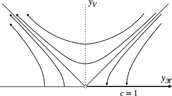
Renormalization Group Flow for Kosterlitz-Thouless Transition — The Kosterlitz-Thouless RG flow diagram. The horizontal axis represents the inverse stiffness $K^{-1}$, which increases with temperature. The vertical axis represents the vortex fugacity $y$. The arrows show how these effective parameters change as we observe the system on larger and larger length scales.

Let's trace the flows:

Low-Temperature Phase ( $T < T_{K T}$ ): The initial stiffness is high, so $K > 2/ π$ . This means $(2 - π K) < 0$ . The second RG equation, $d y / d l < 0$ , tells us that the vortex fugacity $y$ flows towards zero as we increase the length scale. Although small pairs screen the interaction slightly (causing $K^{- 1}$ to increase), the vortices are ultimately irrelevant at large scales. They bind together and "renormalize away". The system flows to a line of fixed points on the horizontal axis ( $y = 0$ ), corresponding to the quasi-long-range ordered phase governed by spin waves.
High-Temperature Phase ( $T > T_{K T}$ ): The initial stiffness is low, so $K < 2/ π$ . This means $(2 - π K) > 0$ . Now, $d y / d l > 0$ . The vortex fugacity grows with length scale. This creates a runaway feedback loop: more vortices create more screening (increasing $K^{- 1}$ ), which further reduces $K$ , which in turn makes it even easier to create more vortices. This is the unbinding transition. The flow runs away to $y \to \infty$ , signifying a proliferation of free vortices that completely disorder the system. This is the disordered phase with short-range correlations.

The separatrix—the special trajectory that divides these two behaviors—corresponds to the critical point itself, $T = T_{K T}$ . It begins at the critical temperature, where the initial stiffness is exactly $K_{c} = 2/ π$ .

Test your understanding!

Imagine you perform an RG transformation on a system that is exactly at the critical temperature $T_{K T}$ . According to the flow diagram, where does the system end up after observing it at an infinitely large length scale ( $l \to \infty$ )? What is the physical meaning of this destination point?

Show answer

A system exactly at $T_{K T}$ lies on the separatrix. Following the flow along this trajectory leads to the fixed point at $(K^{- 1}, y) = (π /2, 0)$ .

This means that at the critical point, the system flows to a state with a finite, universal stiffness $K_{e ff} = 2/ π$ and zero vortex fugacity. The fact that the system flows to a non-trivial fixed point is the hallmark of a continuous phase transition. The value of the stiffness at this fixed point gives rise to the "universal jump" we mentioned in the previous lesson.

Conclusion

Today we have unpacked the intricate mechanism driving the Kosterlitz-Thouless transition. We have moved from a simple picture of pair breaking to a sophisticated understanding based on collective effects.

Key Takeaways:

The mechanism of the KT transition is the collective screening of the logarithmic interaction between vortex-antivortex pairs.
The physics of interacting vortices can be formally mapped onto a 2D Coulomb gas, where vortex charges interact via a logarithmic potential.
The renormalization group (RG) provides the framework to analyze this screening. It shows how the effective interaction strength (stiffness $K$ ) and vortex density (fugacity $y$ ) change with length scale.
At low temperatures ( $T < T_{K T}$ ), the RG flow shows that vortices are irrelevant at large scales, leading to a quasi-ordered phase of bound pairs.
At high temperatures ( $T > T_{K T}$ ), the RG flow runs away, signifying a proliferation of free vortices that screen interactions and drive the system into a disordered phase. The unbinding is therefore a scale-dependent, collective phenomenon.

Preview of the Next Lesson:

Our entire discussion of phase transitions so far—from mean-field theory to the RG analysis of the KT transition—has focused on static, equilibrium properties. However, real systems evolve in time. How does the approach to a critical point affect a system's dynamics? In the next lesson, we will introduce dynamic critical phenomena, exploring concepts like critical slowing down and the dynamic scaling hypothesis.