Critical Slowing Down: Dynamics Near Phase Transitions

Hello! Welcome to our next lesson on advanced topics in critical phenomena.

In our recent lessons, we've explored fascinating aspects of static, equilibrium phase transitions. We dissected the Kosterlitz-Thouless transition, revealing how the unbinding of topological defects drives a phase transition without long-range order. All of our analysis so far—from mean-field theory to the renormalization group—has focused on a system's properties once it has reached thermal equilibrium.

But real systems exist and evolve in time. This raises a crucial question: How does the approach to a critical point affect a system's dynamics? How long does it take for a system to respond to a change or settle into its new equilibrium state? Today, we pivot from the static to the dynamic. Our goal is to introduce dynamic critical phenomena and the concept of critical slowing down near a phase transition. This will lay the groundwork for a more formal scaling theory of dynamics.

1. The Intuitive Picture: Why Things Slow Down

At the heart of static critical phenomena is the divergence of the correlation length, $\xi$. As a system approaches its critical point ($T\to T_c$), patches of the ordered phase grow larger and larger, spanning macroscopic distances.

Now, consider the consequences of this for the system's temporal evolution. For the system to equilibrate or respond to an external perturbation, information must propagate across these enormous, correlated domains. If a spin flips in one part of a correlated cluster, it takes time for its influence to be felt by a spin on the other side of the cluster. As the cluster size $\xi$ blows up, it's natural to expect that this characteristic time will also diverge. This phenomenon is known as critical slowing down.

Another way to visualize this comes from our understanding of Landau theory. A continuous phase transition corresponds to the minimum of the free energy landscape becoming progressively flatter as $T\to T_c$. If you imagine a ball representing the system's state rolling in this potential landscape, a steep well leads to rapid relaxation back to the minimum after a kick. A very flat well, however, provides a much weaker restoring force, causing the ball to roll back incredibly slowly.

In essence, critical slowing down is the temporal signature of an impending critical transition, just as the diverging correlation length is the spatial signature. Experimentally, this manifests as extremely long relaxation times and a dramatic increase in the temporal correlation of fluctuations.

2. Modes of Relaxation: Propagating vs. Relaxational

Before we quantify critical slowing down, it's useful to classify the different ways a system can return to equilibrium. The dynamics of fluctuations, or "modes," generally fall into two categories.

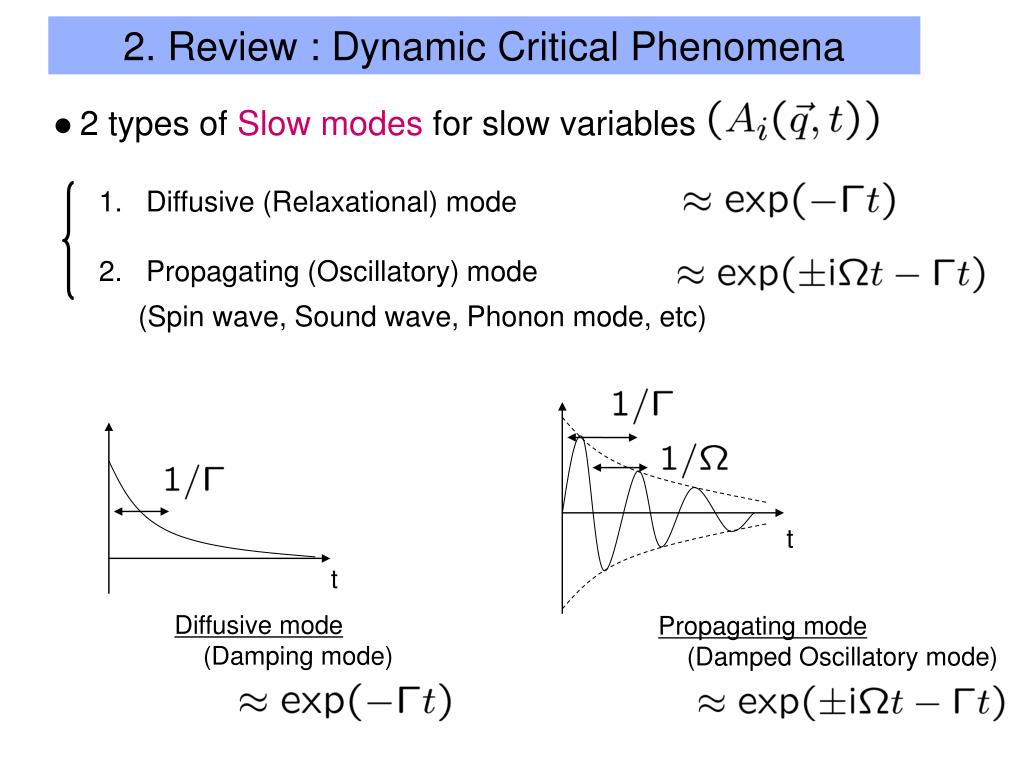
• Propagating Modes: These are oscillatory, like sound waves in a fluid or spin waves (magnons) in a magnet. They have a characteristic frequency $\Omega$ and a damping rate $\Gamma$.
• Relaxational (or Diffusive) Modes: These are purely dissipative and non-oscillatory. A perturbation simply decays back to equilibrium exponentially, characterized by a single relaxation rate $\Gamma$.

While many modes exist in a system, critical phenomena are dominated by the behavior of the "slowest" mode, which is typically the relaxational mode of the order parameter itself. It is the relaxation rate of this critical mode that vanishes at $T_c$.

3. Quantifying Critical Slowing Down: The Dynamic Critical Exponent

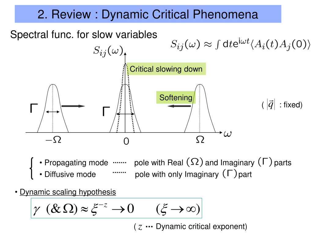
We can now make our intuitive picture precise. We define a characteristic relaxation time, ${\tau }_c$, for the order parameter. Critical slowing down means that this time scale diverges as we approach the critical temperature $t=(T-T_c)/T_c\to 0$.

Just as we related all static divergences to the correlation length $\xi$, we do the same for dynamics. The fundamental ansatz of dynamic critical phenomena is that the characteristic time ${\tau }_c$ scales with the correlation length $\xi$ as:

Here, $z$ is a new, independent exponent called the dynamic critical exponent. It describes the scaling relationship between time and space at criticality. Since we know $\xi \sim |t{|}^{-\nu }$, we can also write the divergence in terms of temperature:

The exponent combination $z\nu$ is often denoted as ${\nu }_t$. The exponent $z$ is as fundamental to dynamics as $\nu$ and $\eta$ are to statics.

The following resource provides a concise, formal introduction to this idea.

We can visualize this phenomenon by looking at the frequency-dependent correlation or response functions. The relaxation time ${\tau }_c$ is inversely proportional to the width $\Gamma$ of the spectral function for a relaxational mode. Critical slowing down (${\tau }_c\to \infty$) implies that this width shrinks to zero ($\Gamma \to 0$).

4. Dynamic Universality Classes: The Role of Conservation Laws

What determines the value of $z$? Like static exponents, $z$ is universal, but it depends not only on dimensionality and order parameter symmetry, but also on the conservation laws governing the dynamics. This gives rise to dynamic universality classes, which are a finer classification than their static counterparts.

A simple way to see this is to consider a time-dependent extension of the Landau-Ginzburg model, often described by a Langevin equation:

Here, $H[S]$ is the familiar Landau-Ginzburg free energy functional, $\zeta$ is a stochastic thermal noise term, and $\mathcal{O}$ is a kinetic operator that dictates the dynamics. The form of $\mathcal{O}$ is crucial.

Let's consider two canonical examples, following the famous classification scheme by Hohenberg and Halperin:

1. Model A (Non-conserved Order Parameter): This describes a system where the order parameter is not a conserved quantity, like the magnetization in an Ising magnet where individual spins can flip freely. In this case, relaxation is a local process. The operator is just a constant kinetic coefficient, $\mathcal{O}=D$.

2. Model B (Conserved Order Parameter): This describes a system where the total order parameter is conserved, such as the density in a liquid-gas transition (atoms can't just appear or disappear). The local density can only change if there is a current flowing, so the dynamics must obey a continuity equation, $\frac{\partial S}{\partial t}+\nabla \cdot \mathbf{j}=0$. This imposes a strong constraint. The relaxation is no longer local but diffusive. This is captured by setting the kinetic operator to $\mathcal{O}=-D^{\prime }{\nabla }^2$.

These two physically distinct situations lead to different values of $z$. For instance, a mean-field analysis (which you can think of as analyzing the Langevin equation in Fourier space and ignoring the non-linear coupling term) yields:

• Model A: $z=2$
• Model B: $z=4$

This demonstrates that conservation laws are a key ingredient in determining the dynamics near a critical point.

Conclusion

Today, we have taken our first step into the rich world of non-equilibrium phenomena at criticality. We moved beyond static snapshots and began to consider how systems evolve in time as they approach a phase transition.

Key Takeaways:

• Critical Slowing Down is the fundamental concept in dynamic critical phenomena. It refers to the divergence of the system's characteristic relaxation time, ${\tau }_c$, as the critical point is approached.
• This divergence is governed by a new, independent dynamic critical exponent, $z$, through the scaling relation ${\tau }_c\sim {\xi }^z$.
• The value of $z$ depends on the dynamic universality class, which is determined not only by static properties (dimension, symmetry) but also by dynamic properties, most importantly the conservation laws of the system.
• Systems with a non-conserved order parameter (like an Ising magnet, Model A) have different dynamic behavior from systems with a conserved order parameter (like a binary alloy or liquid-gas system, Model B).

Preview of the Next Lesson:

We have introduced the dynamic exponent $z$ through the scaling of the characteristic time, ${\tau }_c$. In the next lesson, we will formalize this idea by stating the full dynamic scaling hypothesis. This hypothesis provides a unified scaling form for time- and space-dependent correlation functions and response functions, analogous to the static scaling hypothesis we studied earlier. We will see how $z$ appears naturally in the scaling of frequency and wavevector.