Vector and Matrix Norms

Introduction

In our last lesson, we investigated the determinant, a single number that reveals how a linear transformation scales the space it acts upon. We saw it as a measure of change in area or volume. Today, we shift our focus from the properties of the transformation to the properties of the objects themselves—the vectors and matrices. Our goal is to understand and compute various norms, which are functions that measure the "size," "length," or "magnitude" of these objects.

This lesson will address the learning outcome: Compute and compare L1, L2, and Frobenius norms for vectors and matrices. We'll start from the first principles that define what a norm is, then explore the most common vector and matrix norms, paying close attention to their distinct geometric interpretations and practical implications, particularly in machine learning and optimization. This provides a crucial foundation before we move on to decomposing matrices into their fundamental components.

What is a Norm? The Axiomatic Foundation

Before we start calculating different types of norms, it's essential to establish what properties a function must have to be considered a norm in the first place. Much like how we derived the determinant from a few core axioms about signed volume, we can define a norm by four fundamental rules. A function $f:{\mathbb{R}}^n\to \mathbb{R}$ that maps a vector to a real number is a norm, denoted $\Vert \mathbf{x}\Vert$, if it satisfies these conditions for any vectors $\mathbf{x},\mathbf{y}\in {\mathbb{R}}^n$ and any scalar $t\in \mathbb{R}$.

To see these properties laid out formally, please review this brief section from the Stanford CS229 linear algebra notes.

Any function that satisfies these four axioms can be considered a valid norm. While there are infinitely many such functions, a few stand out for their utility in mathematics and machine learning.

Vector Norms: The $L_p$ Family

The most common vector norms belong to the $L_p$ family, defined by the general formula:

$$\Vert \mathbf{x}{\Vert }_p={\left(\sum _{i=1}^n|x_i{|}^p\right)}^{1/p}$$

By varying the value of $p$, we get different ways of measuring a vector's length. Let's examine the three most important cases: $p=1$, $p=2$, and the limit as $p\to \infty$.

Let's break these down:

1. The $L_2$ Norm (Euclidean Norm):
   When $p=2$, we get the familiar Euclidean distance from the origin.
   $\Vert \mathbf{x}{\Vert }_2=\sqrt{{\sum }_{i=1}^n{x}_i^2}=\sqrt{{\mathbf{x}}^T\mathbf{x}}$
   This is the "as the crow flies" distance and is the most intuitive notion of length.

2. The $L_1$ Norm (Manhattan or Taxicab Norm):
   When $p=1$, the norm is the sum of the absolute values of the components.
   $\Vert \mathbf{x}{\Vert }_1={\sum }_{i=1}^n|x_i|$
   This is called the Manhattan distance because it's analogous to navigating a grid-like street layout, where you can only travel along the axes.

3. The $L_{\infty }$ Norm (Max Norm):
   In the limit as $p\to \infty$, the largest component of the vector dominates the sum. The $L_{\infty }$ norm is simply the maximum absolute value of any element in the vector.
   $\Vert \mathbf{x}{\Vert }_{\infty }={\max }_i|x_i|$

The Geometry of Norms: Unit Balls

The differences between these norms become visually apparent when we plot all the vectors for which the norm is equal to 1. This set of vectors forms the unit ball (or unit circle in 2D) for that norm.

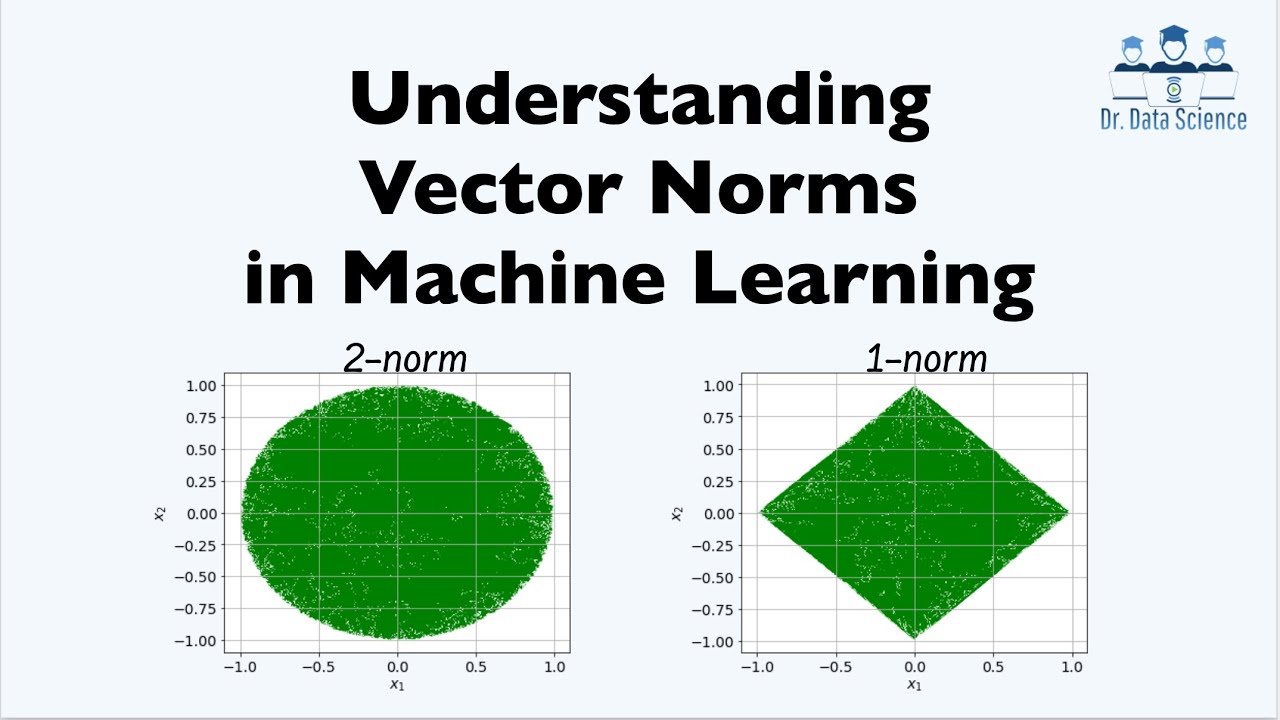
Notice the sharp corners of the $L_1$ unit ball, which lie on the axes. The $L_2$ unit ball, in contrast, is perfectly round.

This next video provides an excellent visualization of how these shapes are formed and how they relate.

The geometric shape of the unit ball is not just a curiosity; it has profound implications for optimization problems, which are at the heart of machine learning.

Consider an optimization problem where we must find the "smallest" vector (as measured by some norm) that also satisfies a linear constraint, like $a{x}_1+b{x}_2=c$. Geometrically, this is like finding the point on a line that is closest to the origin. To find this point, we can imagine inflating the unit ball of our chosen norm until it just touches the line.

Question: Looking at the shapes of the $L_1$ (diamond) and $L_2$ (circle) unit balls, where would you expect the point of contact to be for each norm? How might the "pointiness" of the $L_1$ ball affect the solution you find?

Hint

A smooth, round object like the $L_2$ ball is likely to touch the line at a unique point somewhere in the middle. A pointy object like the $L_1$ ball is more likely to make first contact at one of its corners.

This difference is precisely why the $L_1$ norm is so important in modern machine learning.

This tendency to produce solutions with zero-valued components is called sparsity. By minimizing the $L_1$ norm of a vector of model weights (a technique called L1 regularization or LASSO), we encourage the model to set unimportant weights to exactly zero. This effectively performs feature selection, making the model simpler and more interpretable. The $L_2$ norm, by contrast, prefers to shrink all weights towards zero without making them exactly zero, resulting in a dense solution.

Matrix Norms

Just as we measure the size of vectors, we often need to measure the size of matrices. This is crucial in many areas, for instance, in quantifying the error between a target matrix and its approximation, or analyzing how a transformation amplifies noise.

A key resource for this section is this text, which frames matrix norms from a practical, engineering-oriented perspective.

The Frobenius Norm

The most straightforward way to define a matrix norm is to treat the $m\times n$ matrix as a long vector with $mn$ elements and then calculate its $L_2$ norm. This is called the Frobenius norm.

For a matrix $\mathbf{A}\in {\mathbb{R}}^{m\times n}$, the Frobenius norm is:

$$\Vert \mathbf{A}{\Vert }_F=\sqrt{\sum _{i=1}^m\sum _{j=1}^n{A}_{ij}^2}=\sqrt{\mathrm{tr}({\mathbf{A}}^T\mathbf{A})}$$

The tr denotes the trace of the matrix (the sum of its diagonal elements).

The Frobenius norm measures the "average gain" of the matrix.

Operator Norms: The Matrix 2-Norm

A more sophisticated approach is to define a matrix norm based on how much it can "stretch" a vector. This gives rise to operator norms, which are "induced" by vector norms. The general form is:

$$\Vert \mathbf{A}\Vert =\underset{\Vert \mathbf{x}\Vert =1}{\max }\Vert \mathbf{Ax}\Vert$$

This definition asks: what is the maximum length the output vector $\mathbf{Ax}$ can have, given that the input vector $\mathbf{x}$ has a length of 1?

When the vector norm used is the $L_2$ norm, the induced matrix norm is called the matrix 2-norm or spectral norm. It turns out that this value is precisely the largest singular value (${\sigma }_1$) of the matrix. We will explore singular values in depth in the next module, but for now, the key takeaway is its interpretation.

Conclusion

In this lesson, we have moved from the abstract definition of a norm to a concrete understanding of the most common types used for vectors and matrices.

Key Takeaways:

• Norms as Measures of Size: A norm is a function that assigns a strictly positive "length" to every vector or matrix, with the zero vector/matrix being the only exception.
• Vector $L_p$ Norms: The $L_2$ (Euclidean) norm is our standard notion of distance. The $L_1$ (Manhattan) norm measures path length on a grid and is crucial for promoting sparsity in machine learning models due to the "pointy" shape of its unit ball. The $L_{\infty }$ norm simply captures the largest component.
• Matrix Norms: The Frobenius norm is the matrix equivalent of the vector $L_2$ norm, treating the matrix as a flattened vector. It can be interpreted as the average (RMS) gain of the transformation. The matrix 2-norm (spectral norm) is an operator norm that measures the maximum possible "stretching" factor, or the peak gain, and is vital for worst-case analysis.

Understanding these different ways to measure "size" is fundamental. In optimization, norms define the objective functions we seek to minimize (e.g., minimizing the $L_2$ norm of the error vector in least squares). In regularization, they are added as penalties to prevent model weights from growing too large.

In our next lesson, we will begin a new module on geometric decompositions. We will start with eigenvalues and eigenvectors, which reveal the intrinsic axes of a linear transformation and form the bedrock for understanding more advanced techniques like Singular Value Decomposition (SVD). This will also fully illuminate why the matrix 2-norm is equal to the largest singular value.