Importing Libraries and Calling Functions in Python

Hello! Last lesson, you defined functions and used their returned values. This time, you will call functions that other programmers have already written. You will import a module, use the dot notation to reach one of its functions, and then try the import style commonly used in machine learning notebooks.

Allow about 40 minutes: three minutes for a video, six minutes for reading, and the rest for running and inspecting the code.

A function you did not write

Python provides functions such as print() without an import. Many other functions live in modules: collections of related code that you make available with an import statement. Watch this short introduction for the distinction between a library, a module, and a function. Its example imports a function directly; we will also use the common module.function() form.

Start with math, a module supplied with Python. Run this in a notebook cell:

import math

result = math.sqrt(25)
print(result)

The output is 5.0. You did not define sqrt; the import made the math module available, and math.sqrt(25) called its square-root function with 25 as the argument. Just like a function you write yourself, this call returns a value that can be stored in a variable.

The dot matters. In math.sqrt(25), math identifies where Python should look, while sqrt(25) specifies the function call. The import does not by itself make sqrt(25) available as a standalone call.

Import NumPy using its conventional name

NumPy is a library you will use for numerical data in the next module of this course. Unlike math, it does not come with Python itself, though many machine learning notebook environments already include it. Its documentation shows a widely used import convention:

Now run:

import numpy as np

print(np.ones(3))
print(np.zeros(3))

You should see:

[1. 1. 1.]
[0. 0. 0.]

as np gives the imported library a short name in your code. The convention is useful because you can recognize calls to NumPy functions by their np. prefix. In np.ones(3), the argument 3 requests three elements; np.zeros(3) requests the same number of zeroes.

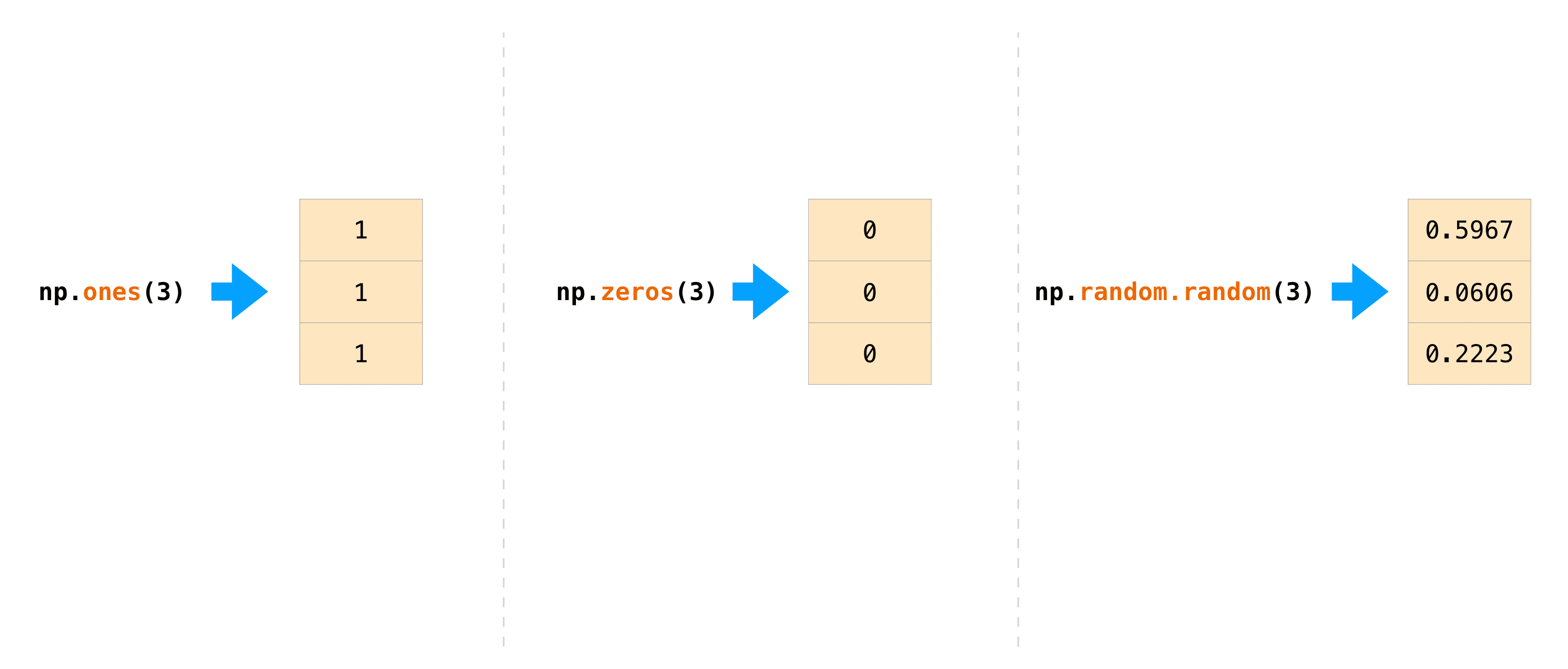
These results are NumPy arrays, not Python lists. For now, focus on importing the library and calling its functions; the next module will examine arrays and arithmetic on them. If you try the image’s np.random.random(3), expect different decimal values from those pictured.

Two import styles, one calling principle

The video used from random import randint, which brings a particular function into the notebook under its own name. You can use the same style with the earlier square-root example:

from math import sqrt

print(sqrt(25))

This prints 5.0 too. Compare the two forms:

Choose the call to match the name you imported. The prefixed form makes a function’s origin visible; the direct form is convenient when you need a particular function. Both still use arguments and returned values in the way you learned last lesson.

A notebook remembers names created by earlier cells. If you run both math examples above, both math.sqrt(25) and sqrt(25) will work afterward. That can hide a missing import when you copy a call into a fresh notebook, so keep the necessary import near the start of your work and run its cell before cells that depend on it.

If import numpy as np reports ModuleNotFoundError, NumPy is not available in that notebook’s Python environment; the import statement does not install it. The math examples still let you use the import-and-call pattern.

Takeaways

Importing makes code from a module available to your notebook. With import math, call a function as math.sqrt(25); with import numpy as np, use the conventional np name, as in np.ones(3). A call to an imported function can return a value just as a call to your own function can.

Next, you will learn to use a traceback to identify which line caused a Python error—a useful skill when an import or function call does not behave as expected.