Recommended resources
The freely available resources this lesson will direct you to.
Hello. In the previous lesson, you traced how inputs and weights produce model scores. The shapes told you whether the computation was possible; they did not tell you whether the scores were good. This lesson adds a way to measure prediction error and adjust one weight to reduce it.
You’ll compute the derivative of a one-parameter loss, use its sign and size to choose an update, and check what happened to the loss. Allow about 35–40 minutes, including the video and time to follow the arithmetic.
From a model score to a loss
Suppose a model uses one numerical feature to predict a numerical target . It has one adjustable parameter, :
Here is the prediction. Unlike the two-score model in the previous lesson, this model produces one prediction per example. The feature values and target values are fixed during an update; is the value we change.
Consider two training examples:
| Example | Feature | Target |
|---|---|---|
| 1 | 1 | 2 |
| 2 | 2 | 4 |
To judge a choice of , we can square each prediction error and take the average. This is mean squared error:
A loss function assigns a number to a parameter choice: lower means better predictions on these examples, according to this particular measure. At , both predictions are zero, so
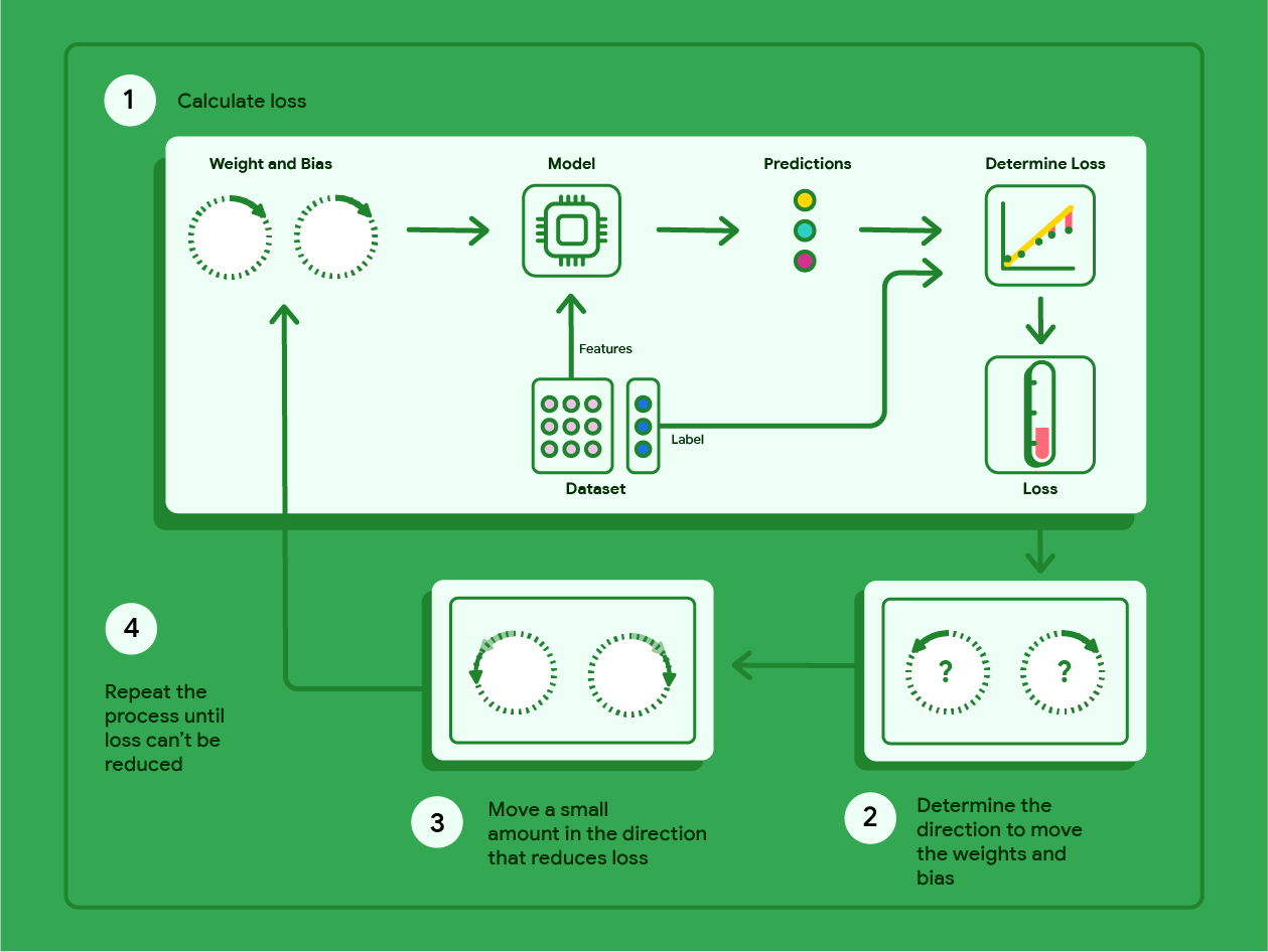
We could try many parameter values and compare their losses. Gradient descent instead uses the slope of the loss at the current value to decide how to move.
What the gradient tells you
With one adjustable number, the gradient is simply the derivative of the loss with respect to that number, written . Imagine a graph with on the horizontal axis and on the vertical axis. The derivative is the graph’s slope at your current .
A positive derivative means that a small increase in would increase the loss, so moving toward smaller values is locally downhill. A negative derivative means that a small increase in would decrease the loss. A derivative of zero means the graph is locally flat; it does not, by itself, guarantee a global minimum for every possible loss function.
Watch the one-parameter portion of Gradient Descent from DeepLearningAI. It uses a parameter named and a loss named ; in our example, these play the roles of and .
DeepLearningAI’s “Gradient Descent” makes the update rule visual: the derivative’s sign determines which way to move along a one-parameter loss curve.
Watch one-parameter descent. Focus on the two starting positions: why subtracting a positive slope moves the parameter left, while subtracting a negative slope moves it right. The video’s cost function is not the same as our worked example, but the update rule is.
To compute the slope for our example, differentiate the loss while treating each and as fixed data. For a single squared error, the chain rule says to differentiate the square and multiply by the derivative of its contents:
The last matters: changing changes the prediction by an amount that depends on the feature value. Applying this rule to both examples gives
This expression is the gradient function. It tells us the slope at any proposed . At our starting value, , the gradient is . Its negative sign tells us to increase if we want to move downhill locally.
Make an update, then check it
Gradient descent scales the gradient by a positive learning rate and subtracts the result from the current parameter:
The vertical bar means evaluate the derivative at the current parameter value. Choose . Starting at , where the gradient is , one update gives
The new predictions are and , rather than and . Recalculating the loss confirms the improvement:
For another update, recompute the gradient at the new value. At , it is , so
Now the predictions are and , and the loss is
The progression is worth noticing: the gradient changed from to . With the same learning rate, the second change to was smaller than the first. In this example, the loss reaches zero at , where the derivative is also zero.
The learning rate controls more than speed. If we instead used for the first update, the same starting gradient would give . Its predictions would be and , producing a loss of —worse than the starting loss of . Subtracting the gradient does not guarantee that every step reduces loss: a step can be too large and overshoot. A very small learning rate avoids large moves but may require many updates.
For this particular quadratic loss, you can see the destination directly by simplifying it:
Gradient descent does not need us to solve for that destination first. Its useful procedure is to calculate the slope where we are now, update, and calculate again.
The reusable training loop
Our calculation illustrates a general procedure without requiring a more complex model:
- Choose an initial parameter and calculate predictions and loss on the training examples.
- Differentiate the loss with respect to the parameter, then evaluate that derivative at its current value.
- Subtract the learning rate multiplied by that gradient.
- Recalculate at the updated value and repeat, while monitoring whether the loss is improving.
In practice, training can stop after a set number of updates or when changes become sufficiently small. Monitoring matters: a tiny update might mean you are near a flat region, but it can also result from a very small learning rate. Likewise, reducing training loss says how well the model fits the data used for its updates, not yet how well it will perform on new data.
The central calculation is now in place: derive the loss slope, evaluate it at the current parameter, and subtract a suitably scaled version of it. Next, you’ll use conditional probability, expectation, and variance to interpret what a model prediction means—an important distinction from merely making its training loss smaller.