Recommended resources
The freely available resources this lesson will direct you to.
Hello. Last lesson, you changed a model parameter to reduce prediction error. A lower training loss tells you the model fit those examples better, but it does not yet tell you how to interpret a prediction such as “0.30” or “1.7.”
This lesson separates three ideas: conditional probability describes how likely an outcome is given the available inputs; expectation describes the average outcome under those conditions; and variance describes how widely outcomes can differ from that average. Together, they help you distinguish a model’s estimate from the outcome that will actually occur. Allow about 40 minutes, including the short video and readings.
What does “given these inputs” mean?
Imagine a model that predicts whether a request will need specialist review. Let mean that review is needed and mean it is not. For now, let record whether the request has a particular characteristic: if it does, otherwise.
Suppose we could observe the following counts in a population:
| Request characteristic | Needs review | Does not need review | Total |
|---|---|---|---|
| 60 | 140 | 200 | |
| 80 | 720 | 800 |
Across all requests, the proportion needing review is . But once we know that a request has , the relevant group contains only 200 requests. Within that group, the proportion needing review is . We write this conditional probability as
The vertical bar means “given.” It changes the group we are considering, and therefore the denominator. Reversing the condition asks a different question: , not .
For a general event given an event , the definition is
Read the “Conditional Probability” section of Seeing Theory for a second way to picture why the denominator changes. Its coin example introduces new information; its shelf illustration treats the known condition as the new space within which to count.
Read the “Conditional Probability” section of Seeing Theory to reinforce what the word “given” does to a probability.
In the “Conditional Probability” subsection of “compound probability” (p. 27), begin with the coin example at the coin and shelf examples. Stop after the shelf illustration, before the “Bayes Rule” subsection on p. 28. Focus on which possibilities remain in the denominator after the new information is known.
In a real application, we do not know the population probability from a complete table. A model uses observed data to estimate the probability of for supplied features , often written . If it outputs , the intended interpretation is that among comparable requests assigned probabilities near 0.30, roughly 30% would need review—if the estimate is well calibrated. It does not mean that this particular request is “30% of the way” toward needing review.
Expectation: the average outcome, not a guaranteed outcome
An expected value weights each possible numerical outcome by its probability. Watch how Expected Values, Main Ideas!!! by StatQuest develops this from a wager: the average gain can be an amount that no single wager pays.
Expected Values, Main Ideas!!!
Watch Expected Values, Main Ideas!!! from StatQuest with Josh Starmer for the repeated-outcomes intuition behind an expected value.
Start at the wager, where the video combines likely wins and losses. Continue through expected value, where it turns that calculation into an average per wager. Focus on the distinction between a possible single result and an average across repeated results.
For our binary request outcome, suppose the conditional probability is . Given , the only possible values of are zero and one, so its conditional expectation is
No individual request has an outcome of 0.30: its observed outcome will be either zero or one. The value 0.30 is the average of the zero–one outcomes we would expect across requests with those conditions. For a zero–one target, conditional expectation and the probability of one are the same number.
For a numerical target, expectation works the same way, but it need not be a probability. Suppose a model’s estimated distribution for the number of follow-up contacts is:
| Contacts | Estimated probability given |
|---|---|
| 0 | 0.20 |
| 1 | 0.50 |
| 4 | 0.30 |
The expected count is
“1.7 contacts” is a meaningful average prediction, even though no request can generate exactly 1.7 contacts.
There is a direct connection to the squared-error loss you used last lesson. If you must make one numerical prediction for all cases with the same information , the conditional mean is the value that minimizes expected squared error. The short reading below makes that connection explicit.
28 Conditional Expectations and Smoothing – Introduction to Data Science
Read the end of Section 28.1 and the beginning of Section 28.2 in Introduction to Data Science. They connect binary probabilities to conditional means, then connect conditional means to the squared-error criterion.
In Section 28.1, “Conditional probabilities and expectations,” start at the binary interpretation; include the displayed equation immediately following it at the start of Section 28.2. Then, in Section 28.2, “Conditional expectations minimize the squared loss function,” read from the squared-loss connection, including the displayed minimization statement and the definition of the prediction function. Focus on what the conditional mean minimizes—not on the later discussion of possible function shapes.
Why does the mean minimize squared error? Call the conditional mean . For any proposed prediction ,
The first term does not change when you change ; the second is smallest at . Training a model on squared error is therefore a way to try to estimate a conditional mean. It cannot make every outcome equal that mean.
Variance: how much remains uncertain about the outcome?
A mean alone can conceal substantial differences among possible outcomes. Conditional variance measures the average squared distance of from its conditional mean:
Read the opening of the “Variance” subsection in Seeing Theory. Notice why simply averaging signed differences from the mean would not measure spread: positive and negative differences cancel.
Return to Seeing Theory for the definition of variance and the reason it uses squared differences.
In “basic probability,” find the “Variance” subsection on pp. 12–13. Read from the variance explanation, stopping before the proposition and its proofs. Focus on the distance from the mean and why that distance is squared.
For the binary requests with , the mean is . We can calculate the variance by considering both possible outcomes:
More generally, when a zero–one outcome has conditional probability of being one, its conditional variance is . The square root is the standard deviation; here it is approximately , expressed in units of the zero–one outcome.
For the numerical contacts example, the mean was 1.7. Its conditional variance is
The standard deviation is about contacts. That spread matters when interpreting the prediction “1.7”: four contacts remains a possible outcome, with an estimated probability of 0.30. The mean identifies a center; the distribution and variance tell you more about what might happen around it.
Keep two kinds of uncertainty separate. Conditional variance describes variation in the outcome among cases with the given features. It is not the variance of the model’s single output for this request, nor does it quantify how uncertain we are about whether the model learned the correct probabilities from limited data.
Interpreting a model’s number responsibly
A model output displayed between zero and one is not automatically a trustworthy probability. For instance, a model might assign 0.80 to a collection of cases in which only 60% actually have the outcome. Its numbers would then be too high for that group. Checking whether predicted probabilities agree with observed frequencies is called calibration.
The plot below makes that distinction visible. In its top panel, the dotted diagonal represents agreement between a group’s mean predicted probability on the horizontal axis and its observed fraction of positive outcomes on the vertical axis. A curve closer to that diagonal indicates better agreement in the plotted groups. The histograms underneath show how frequently different probabilities were predicted; their shape alone does not establish whether the predictions were correct.
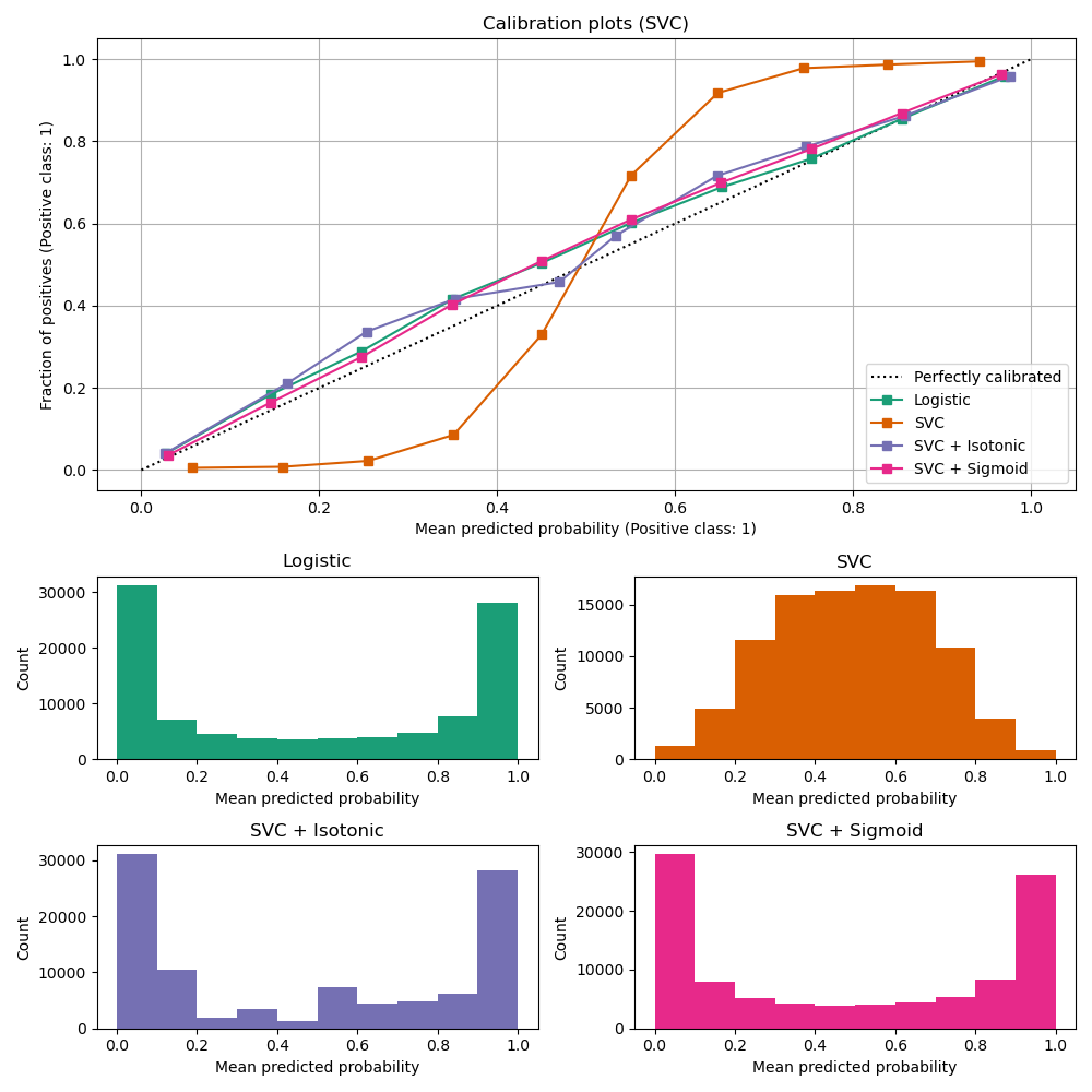
Here, the uncalibrated SVC curve departs markedly from the diagonal, while its calibrated variants track it more closely in the displayed plot. That does not establish that one technique is always reliable, or prove the probability of an individual case. It shows why interpreting “0.80” as “about eight in ten comparable cases” requires evidence about the model’s probabilities, ideally on data not used to fit them.
Finally, a probability is information for a decision, not the decision itself. Return to the request with an estimated 0.30 chance of needing review. Suppose an unnecessary review has a cost of 1 unit, while failing to review a request that needs it has a cost of 4 units. Under these simplified assumptions, the expected cost of reviewing is ; the expected cost of not reviewing is . Review has the lower expected cost despite the outcome being less likely than not. The decision depends on consequences as well as probabilities—a topic you will develop further when choosing evaluation metrics and, later, classification thresholds.
Key takeaways
A prediction should be read in light of what is conditioned on and what quantity is being predicted. Conditional probability concerns an outcome given inputs. Conditional expectation is the average numerical outcome under those inputs; for a zero–one target, it equals the probability of one. Conditional variance describes outcome spread around that mean, not uncertainty about whether the model itself is correctly estimated. And when a model reports a probability, calibration matters before you treat that number as a dependable frequency.
Next, you’ll consider how to separate training, validation, and test data so that estimates of model performance are not distorted by information the model should never have seen.