Determining Vector and Matrix Shapes in Simple Models

Hello. Last time, you separated an AI system’s input, model output, decision, and success criterion. Now we’ll look inside a simple model computation. Its inputs and parameters are arranged as vectors and matrices, and their shapes determine which calculations are possible—and how many outputs the model produces.

By the end of this lesson, you should be able to look at a computation such as $XW+b$, identify the shape of each part, and determine the shape of the result. Allow about 40 minutes for the lesson, including the videos and reading.

Count rows and columns first

A vector is an ordered collection of numbers. For example, three numerical features describing one support request might form the vector $[2,1,0]$. A matrix arranges numbers in rows and columns. If each row describes one request and each column represents one feature, two requests with three features each form a matrix with 2 rows and 3 columns, written $2\times 3$.

Watch Greg Hogg introduce vectors and matrices before we use them in a model calculation.

Suppose our feature matrix is

Its shape is $2\times 3$. The first row describes one request; the second describes another. The three columns must represent the same three features in the same order for both requests. Shape tells us how the numbers are arranged, but not what they mean.

The image below shows why that distinction matters. The same six numbers can fit into either arrangement, but a $2\times 3$ matrix and a $3\times 2$ matrix would imply different numbers of examples and features in our dataset.

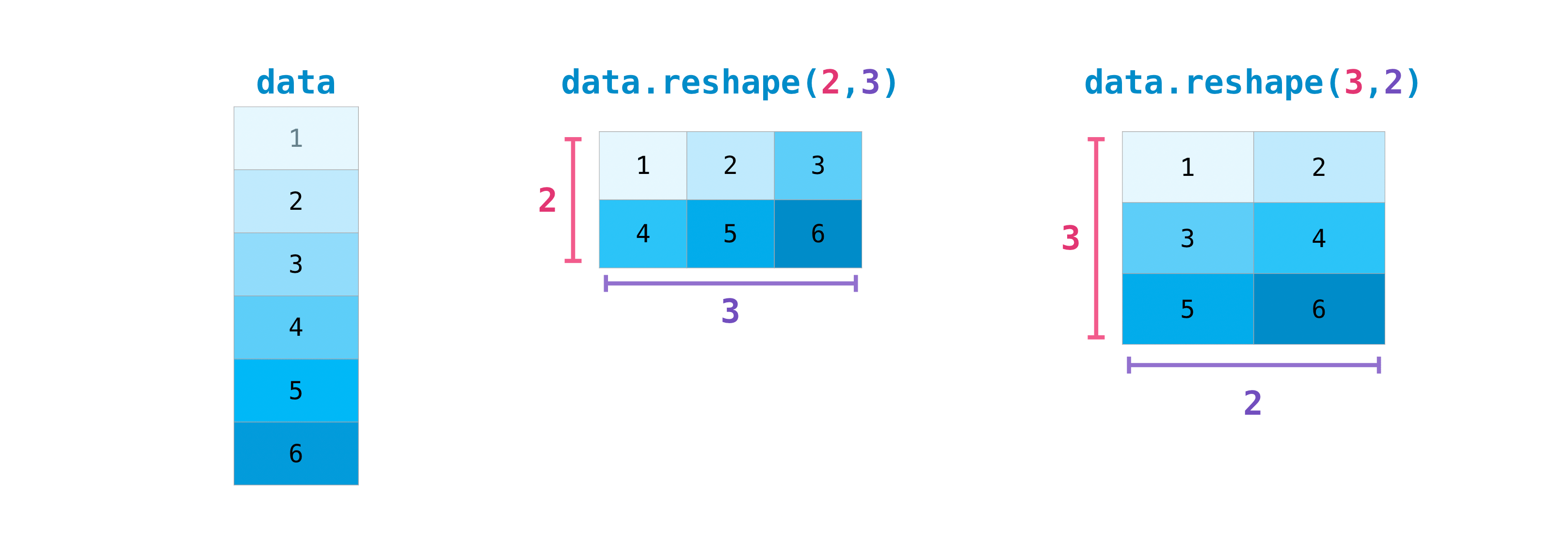
A single three-feature example can be written as a row vector of shape $1\times 3$, or as a column vector of shape $3\times 1$. Those orientations are not interchangeable in multiplication. In NumPy, an ordinary one-dimensional array of three values has shape $(3,)$: it has three entries but does not itself have a row or column axis. When orientation matters, make the intended row or column shape explicit.

Multiplication has a shape requirement

To understand matrix multiplication, start with a dot product: pair corresponding entries, multiply each pair, and add the products. For instance, the row $[2,1,0]$ and a column containing $1,-1,2$ produce $2(1)+1(-1)+0(2)=1$. Both must contain three entries so that every entry has a partner.

Greg Hogg demonstrates that same operation for every row of a matrix. Watch the dot-product explanation, then the matrix–vector example.

The same principle works when the right-hand side has several columns. Khan Academy’s article makes the general shape rule explicit.

Here is the rule in compact form:

The two inner counts must match: each row on the left has $n$ entries, and each column on the right has $n$ entries. The outer counts give the result: $m$ rows and $k$ columns. If the inner counts differ, ordinary matrix multiplication is not defined. The order matters; reversing the matrices can produce a different shape or make the multiplication impossible.

This rule is a check on structure, not a substitute for meaning. A calculation can have compatible shapes even if its columns represent the wrong features in the wrong order.

Trace one model computation

In the previous lesson’s support-request example, a model might use request features to produce scores that inform routing. We can trace the shapes of a small scoring calculation without needing to decide yet how those scores become actions.

In the following StatQuest excerpt, one input row is multiplied by a matrix of weights—coefficients the model uses for its calculations—and then bias values are added. The excerpt uses two input features and two resulting values.

Now extend that arrangement to our two requests, each with three features. Suppose we want two scores per request. We need a weight matrix with three rows—one for each input feature—and two columns—one for each output score:

Before calculating any values, check the shapes: $X$ is $2\times 3$, and $W$ is $3\times 2$. The inner counts match, so $XW$ has shape $2\times 2$: two requests, each with two scores.

The values confirm what the shapes predicted. The first result entry pairs the first request’s three features with the first weight column:

Doing the same row-by-column calculation for all four entries gives

Suppose the two output scores also have biases $b=[0.5,-1]$. There is one bias per output column, not one per request. To add biases using ordinary matrix addition, repeat that row for each request:

Here $XW$ and $B$ are both $2\times 2$, so their entries can be added position by position. Array libraries often perform that row repetition automatically: they can broadcast a bias row of shape $1\times 2$ across the $2\times 2$ result. That is a library convenience, not a change to the matrix-multiplication rule.

If we wanted one score per request instead, the weight matrix would have shape $3\times 1$. With the same $2\times 3$ input matrix, the result would be $2\times 1$. Notice how changing the number of weight columns changes the number of outputs for each example, while changing the number of input rows changes how many examples are processed.

These numbers are scores, not automatically probabilities, classifications, or routing decisions. Those interpretations require further choices. For now, shapes let you verify that the model produces the intended number of values for the intended number of requests.

Keep the shape contract in view

When tracing a model calculation, identify what each axis represents: examples, features, or outputs. For a batch with $m$ examples, $n$ features, and $k$ outputs per example, the input has shape $m\times n$, the weights have shape $n\times k$, and the product has shape $m\times k$. Biases must supply one value per output and be added in a shape-compatible way.

This habit catches errors before you inspect any arithmetic. In the next lesson, you’ll examine how a model changes a parameter to reduce a loss. Today’s shape checks tell you which computations are possible; the next lesson asks how their values can improve.