Eigenvalue Decomposition of Covariance Matrices

Recommended resources

The freely available resources this lesson will direct you to.

Welcome back to our exploration of the mathematical foundations of machine learning. In our previous session, we delved into the calculus behind model optimization, establishing how gradients and the chain rule form the engine of learning algorithms like backpropagation. Today, we shift our focus to another essential mathematical pillar: linear algebra. We will investigate how the structure of data can be understood and manipulated through matrix operations.

This lesson centers on one of the most elegant concepts in linear algebra and its direct application in data science: eigenvalue decomposition. You will learn to apply this decomposition to a covariance matrix, a statistical construct that describes the shape of a dataset. By the end of this lesson, you will be able to interpret the powerful geometric meaning of this operation and understand how it provides a principled method for data analysis and dimensionality reduction.

The Covariance Matrix: Quantifying the Shape of Data

Before we can analyze the structure of data, we must first have a way to describe it numerically. For a single variable, its variance measures the spread or dispersion around its mean. However, most datasets involve multiple variables, or features. We are often interested not just in how each variable spreads out individually, but also in how they vary together.

This is where covariance comes in. Covariance measures the joint variability of two random variables.

A positive covariance indicates that as one variable increases, the other tends to increase as well.
A negative covariance indicates that as one variable increases, the other tends to decrease.
A covariance near zero suggests little to no linear relationship between the variables.

For a dataset with $d$ features, we can compute the variance of each feature and the covariance between every pair of features. These values are organized into a $d \times d$ covariance matrix, typically denoted by $Σ$ .

Σ = Var (X_{1}) Cov (X_{2}, X_{1}) ⋮ Cov (X_{d}, X_{1}) Cov (X_{1}, X_{2}) Var (X_{2}) ⋮ Cov (X_{d}, X_{2}) \dots \dots ⋱ \dots Cov (X_{1}, X_{d}) Cov (X_{2}, X_{d}) ⋮ Var (X_{d})

The diagonal entries of $Σ$ are the variances of each feature, while the off-diagonal entries $Σ_{ij}$ are the covariances between features $i$ and $j$ . Since $Cov (X_{i}, X_{j}) = Cov (X_{j}, X_{i})$ , the covariance matrix is always symmetric. Fundamentally, the covariance matrix provides a compact, mathematical description of the shape and orientation of a cloud of data points.

A geometric interpretation of the covariance matrix

This article provides an excellent intuition for how the covariance matrix captures the shape of a data distribution.

Please read the introductory section, starting from the beginning. Pay close attention to Figure 2 and Figure 3, which visually demonstrate how the values in the covariance matrix (variances on the diagonal, covariances off-diagonal) correspond to the spread and orientation of 2D data.

Eigenvectors and Eigenvalues: The Intrinsic Directions of a Transformation

Now that we have a matrix ( $Σ$ ) that describes our data's shape, we need a tool to extract the most meaningful information from it. That tool is eigenvalue decomposition.

From a geometric perspective, a matrix represents a linear transformation of space. When we apply a matrix to a vector, the vector is typically rotated and scaled. However, for any given transformation, there may exist special vectors that are not rotated; they are only scaled. These special vectors are the eigenvectors of the matrix. The factor by which each eigenvector is scaled is its corresponding eigenvalue.

This relationship is captured by the defining equation:

A v = λ v

Here, $A$ is the matrix representing the transformation, $v$ is an eigenvector, and $λ$ is its scalar eigenvalue. The eigenvector $v$ simply gets stretched or compressed by a factor of $λ$ when transformed by $A$ , but its direction remains on the same line (its "span").

Eigenvectors and eigenvalues | Chapter 14, Essence of linear algebra

The channel 3Blue1Brown provides one of the best visual intuitions for linear algebra concepts. This video explains what eigenvectors and eigenvalues represent geometrically.

Please watch the following segments to refresh your understanding: Conceptual Introduction (watch here): This part introduces the core idea of eigenvectors as vectors that stay on their own span during a transformation. Why They Matter (watch here): A brief glimpse into why finding these special vectors is so useful, for example, in identifying an axis of rotation. The Computation (watch here): This segment explains the derivation of the characteristic equation, \det(A - \lambda I)\mathbf{v} = \mathbf{0}, which is the standard method for computing eigenvalues and eigenvectors.

Decomposing the Covariance Matrix: Data, Geometry, and Meaning

We can now bring these two concepts together. What do we learn by finding the eigenvectors and eigenvalues of the covariance matrix $Σ$ ?

Since $Σ$ describes the shape of our data, its eigenvectors and eigenvalues reveal the data's intrinsic geometry. Specifically:

The eigenvectors of the covariance matrix are a set of orthogonal vectors that point in the directions of maximum variance in the data. They form a new coordinate system aligned with the data's natural shape. The first eigenvector points in the direction of the greatest variance, the second points in the direction of the second-greatest variance (orthogonal to the first), and so on. These are often called the principal axes of the data.
The eigenvalues tell us the magnitude of the variance along each of these principal axes. The eigenvalue $λ_{i}$ is the variance of the data projected onto the corresponding eigenvector $v_{i}$ .

This decomposition gives us a profound insight: any data distribution can be seen as a simple, uncorrelated spherical distribution (called "white data") that has been scaled and rotated into the shape we observe. The eigendecomposition of the covariance matrix tells us exactly what that scaling and rotation is.

This image illustrates the core idea. A linear transformation can be decomposed into a rotation and a scaling. Panel (a) shows an identity transformation on a unit circle (uncorrelated "white" data). Panel (b) shows scaling along the axes, turning the circle into an axis-aligned ellipse. The scaling factors are the eigenvalues $\lambda_1$ and $\lambda_2$. Panel (c) adds a rotation, orienting the ellipse in a new direction. The eigenvectors of the final transformation matrix define the directions of the ellipse's major and minor axes, and the eigenvalues define their lengths.

The eigendecomposition of a symmetric matrix like $Σ$ is written as:

Σ = V Λ V^{- 1}

Since $Σ$ is symmetric, its eigenvectors are orthogonal, which means the matrix $V$ (whose columns are the eigenvectors) is an orthogonal matrix. For an orthogonal matrix, its inverse is simply its transpose, so $V^{- 1} = V^{T}$ . This gives us:

Σ = V Λ V^{T}

Here:

$V$ is the rotation matrix whose columns are the eigenvectors (the principal axes).
$Λ$ (Lambda) is a diagonal matrix containing the eigenvalues on its diagonal. This represents the scaling (variance) along those principal axes.

A geometric interpretation of the covariance matrix

This article brilliantly connects the mathematical decomposition to a clear geometric process.

Please continue reading from the section Eigendecomposition of a covariance matrix. Read the first part, which explains how eigenvectors point in the direction of largest variance and eigenvalues represent the magnitude of that variance. Next, read the section "Covariance matrix as a linear transformation". This is the key section. It formally shows how the covariance matrix \Sigma can be decomposed into rotation (V) and scaling (\Lambda) matrices and how this relates to transforming uncorrelated "white" data into the observed data distribution. Finally, read the short Conclusion to solidify the main takeaway.

Application: Principal Component Analysis (PCA)

The direct application of this entire process in machine learning is an algorithm called Principal Component Analysis (PCA). PCA is a cornerstone of unsupervised learning and data preprocessing, used primarily for dimensionality reduction.

The goal of dimensionality reduction is to represent a high-dimensional dataset in a lower-dimensional space while preserving as much of the original information (i.e., variance) as possible. PCA achieves this by finding the principal components (the eigenvectors of the covariance matrix) and projecting the data onto the subspace spanned by the components with the largest eigenvalues.

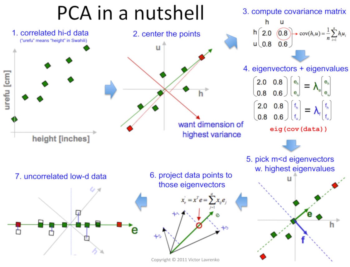
The algorithm for PCA is a direct implementation of the concepts we've just discussed:

Mean-Center the Data: Subtract the mean of each feature from all data points. This shifts the data cloud so its center is at the origin.
Compute the Covariance Matrix: Calculate the covariance matrix $Σ$ of the mean-centered data.
Perform Eigendecomposition: Compute the eigenvectors and eigenvalues of $Σ$ . The eigenvectors are the Principal Components.
Select Components: Sort the eigenvectors in descending order of their corresponding eigenvalues. The eigenvalue $λ_{i}$ represents the variance explained by the $i$ -th principal component.
Project the Data: To reduce the dimensionality from $d$ to $k$ (where $k < d$ ), form a projection matrix $W$ from the first $k$ eigenvectors. The new, lower-dimensional dataset $Z$ is obtained by projecting the original mean-centered data $X$ onto this new basis: $Z = X W$ .

This diagram provides a step-by-step visual summary of the PCA algorithm. It starts with correlated data (1), centers it (2), computes the covariance matrix (3), finds its eigenvectors and eigenvalues (4), selects the top components (5), projects the data onto them (6), resulting in a lower-dimensional, uncorrelated representation (7).

The following resources provide a more formal walkthrough of the PCA procedure.

[PDF] Lecture 14: Principal Component Analysis

This document provides a concise, formal description of PCA.

Please read the following sections: Start with the introduction to understand the goal of PCA. Then, read this section, which explicitly states that the principal components are the eigenvectors of the covariance matrix. The section on the matrix equation shows the formal decomposition \Sigma = \Phi \Lambda \Phi^T, which should now be familiar. Review Figure 3 and the accompanying text in "PCA in practice" for a geometric illustration. Finally, quickly scan the "Dimension Reduction" section, focusing on how the covariance matrix is computed from the data matrix U as \Sigma = U^T U / (N-1) and how the top eigenvectors are selected to form the projection matrix.

To see this workflow described in a video format, including the critical mean-centering step, you can watch the following.

Principal Component Analysis (PCA)

This video by Prof. Steve Brunton explains PCA as a statistical interpretation of matrix decomposition.

This video covers the entire workflow. You can watch it at a higher speed, as the concepts will be familiar. Focus on these key stages: The Goal (watch here): PCA provides a data-driven hierarchical coordinate system. Mean-Centering (watch here): The crucial first step of subtracting the mean. Covariance Matrix (watch here): Computing C = B^T B from the mean-centered data B. Eigendecomposition (watch here): Finding the eigenvectors V (the principal components) of the covariance matrix. Explained Variance (watch here): How eigenvalues (\lambda_k) tell you the fraction of total variance captured by each component. Geometric View (watch here): A summary of how PCA finds the principal axes of the data ellipsoid.

Conclusion

In this lesson, we connected statistics and linear algebra to uncover one of the most fundamental techniques in data analysis. You have seen how a matrix can not only perform a transformation but also describe the very fabric of a dataset.

Here are the key takeaways:

The covariance matrix $Σ$ is a symmetric matrix that numerically captures the shape, spread, and orientation of multidimensional data.
Eigenvalue decomposition breaks down a matrix into its intrinsic components: a rotation (eigenvectors $V$ ) and a scaling (eigenvalues $Λ$ ).
Applying eigendecomposition to the covariance matrix ( $Σ = V Λ V^{T}$ ) reveals the principal axes of variance in the data. The eigenvectors are these axes, and the eigenvalues quantify the amount of variance along each axis.
Principal Component Analysis (PCA) is the algorithmic embodiment of this principle, used for dimensionality reduction by projecting data onto the few principal components that capture the most variance.

We have now added a powerful linear algebra tool to our mathematical arsenal, complementing the calculus we covered previously. In the next lesson, we will introduce a core statistical principle that underpins how we fit most machine learning models to data: Maximum Likelihood Estimation (MLE). This will serve as a bridge from our mathematical groundwork to the practical art of model fitting.