Gradients and the Chain Rule for ML Optimization

Recommended resources

The freely available resources this lesson will direct you to.

In our last lesson, we explored Bayes' theorem as a principled way to update our beliefs about the world given new data. This gave us a powerful theoretical foundation for classification. However, the models we discussed, like Naive Bayes, rely on parameters that we must estimate from data. This brings us to a central question in machine learning: how do we find the best parameters for our models? The answer lies in optimization. We typically define a loss function that measures how "wrong" our model's predictions are, and our goal is to adjust the model's parameters to make this loss as small as possible.

This lesson introduces the core mathematical engine that drives this optimization process: the gradient. We will revisit the fundamentals of multivariable calculus, specifically focusing on how to compute gradients of functions with many inputs and how to handle the complex, nested functions that are characteristic of modern machine learning models using the chain rule. Your strong mathematical and computer science background will be an asset here, as we can treat these concepts with the theoretical rigor they deserve, connecting them directly to their application in training algorithms.

Gradients and Direction of Steepest Descent

In machine learning, we often visualize the loss function as a high-dimensional surface. The parameters of our model (e.g., weights and biases) correspond to a location on this surface, and the height of the surface at that point is the loss. Our goal is to find the lowest point in this landscape.

The most fundamental tool for navigating this surface is the gradient. Let's first build an intuition for what a gradient represents.

Best Explanation of Partial Derivatives and Gradients

This video provides a clear, visual introduction to partial derivatives and gradients using the analogy of a temperature map.

Please watch the first four minutes of the video, covering these segments: The initial analogy of a temperature map and its 3D representation as a hill. The explanation of partial derivatives as slopes in specific directions (e.g., only along the x-axis or y-axis). The definition of the gradient as a vector that combines these partial derivatives to point in the direction of steepest ascent.

As the video explains, for a multivariable function $L (w)$ , where $w$ is a vector of parameters $[w_{1}, w_{2}, \dots, w_{N}]$ , the partial derivative $\frac{\partial L}{\partial w _{i}}$ measures how the function's value changes with a small perturbation in a single parameter $w_{i}$ , while all other parameters are held constant.

The gradient, denoted $\nabla L (w)$ , is simply the vector of all these partial derivatives:

\nabla L (w) = [\frac{\partial L}{\partial w _{1}}, \frac{\partial L}{\partial w _{2}}, \dots, \frac{\partial L}{\partial w _{N}}]^{⊤}

The crucial insight for optimization is that the gradient vector $\nabla L (w)$ always points in the direction of the steepest ascent at point $w$ . Consequently, the negative gradient, $- \nabla L (w)$ , points in the direction of steepest descent. This gives us a clear strategy for minimizing the loss: start at some random point $w$ and iteratively take small steps in the direction of the negative gradient. This is the core idea of the gradient descent algorithm, which we will explore in detail in a future lesson.

Let's formalize this with a reading from the "Dive into Deep Learning" textbook.

18.4. Multivariable Calculus

This resource provides a formal mathematical treatment of gradients and their geometric interpretation in the context of deep learning.

Please read the first two subsections of the chapter: Higher-Dimensional Differentiation: Start reading at the beginning of this section and continue to the definition of the gradient vector in equation (18.4.4). Focus on how the change in a multivariable function is approximated by the dot product of the perturbation vector \boldsymbol{\epsilon} and the gradient \nabla L. Geometry of Gradients and Gradient Descent: Read this entire section, starting from this point. It formally demonstrates why the negative gradient represents the direction of steepest descent.

The Chain Rule for Composite Functions

Neural networks are essentially giant composite functions. The output of the network (and thus the loss) is a function of the activations in the final layer. These activations are a function of the weights and the activations of the previous layer, which are themselves functions of earlier layers, and so on.

To find the gradient of the loss with respect to a weight deep inside the network, we need a way to differentiate through this entire chain of functions. This is where the multivariate chain rule becomes indispensable.

Let's begin with a visual explanation of how the chain rule extends from single-variable functions to the multivariate case.

The Chain Rule for Partial Derivatives — Topic 73 of Machine Learning Foundations

This video by Jon Krohn uses variable flow diagrams to build an excellent intuition for the multivariate chain rule.

Please watch the following segments: Start with the first multivariate example, where the output y depends on a single intermediate function u. Notice how the derivative with respect to an input x is found by "traveling" along the path y -> u -> x. Next, watch the more complex example where the output y depends on multiple intermediate functions u and v. The key insight here is that the total influence of an input x on the output y is the sum of its influences through all possible paths (the u path and the v path). Finally, observe the general formula, which formalizes this idea of summing over all intermediate paths.

The core principle, as the video illustrates, is that the influence of a variable deep within a nested function on the final output is the sum of its influence propagated through every possible path in the computational graph.

If we have $y = f (u_{1}, u_{2}, \dots, u_{m})$ and each $u_{j}$ is a function of $x_{1}, x_{2}, \dots, x_{n}$ , then the partial derivative of $y$ with respect to some input $x_{i}$ is given by:

\frac{\partial y}{\partial x _{i}} = j = 1 \sum m \frac{\partial y}{\partial u _{j}} \frac{\partial u _{j}}{\partial x _{i}}

This formula is the heart of the backpropagation algorithm.

Application: Backpropagation as Applied Chain Rule

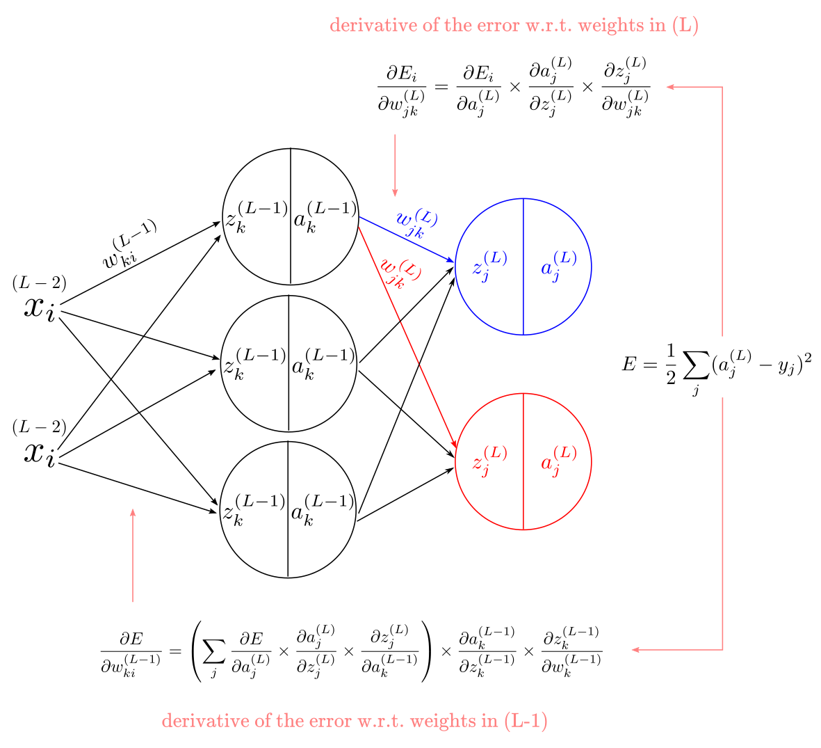
Backpropagation is not a new or distinct mathematical concept; it is simply a clever and computationally efficient algorithm for applying the multivariate chain rule to a neural network. Its purpose is to calculate the gradient of the loss function with respect to every single weight and bias in the network.

From a computer science perspective, you can think of a neural network's computation as a computational graph, where nodes represent variables (parameters, inputs, activations) and edges represent operations (matrix multiplication, activation functions). The process has two phases:

Forward Pass: We start with the inputs and parameters and compute the values of all nodes layer by layer, moving forward through the graph until we calculate the final loss.
Backward Pass (Backpropagation): We start from the end (the loss function) and apply the chain rule recursively, moving backward through the graph. We compute the gradient of the loss with respect to each node, reusing previously computed gradients.

Let's see how this works in a single layer.

This diagram illustrates the forward and backward pass for a single linear layer. In the forward pass, the input `x` is multiplied by the weight matrix `W` to produce the output `y`. In the backward pass, the gradient of the loss with respect to the output, ∂L/∂y, is multiplied by the transpose of the weight matrix, Wᵀ, to propagate the gradient back to the input, yielding ∂L/∂x. This transposition is a direct consequence of the multivariate chain rule applied to matrix-vector operations.

The crucial step is propagating the gradient backward. The gradient of the loss with respect to the layer's input $x$ is found by multiplying the "upstream" gradient (the gradient with respect to the layer's output $y$ ) by the derivative of the layer's function. For a linear layer $y = W x$ , this derivative turns out to be the transposed weight matrix $W^{⊤}$ .

This process is then applied recursively, layer by layer, from the output of the network all the way back to the input.

This diagram shows the recursive nature of backpropagation. The gradient of the error `E` with respect to a weight `w_jk` in layer `L` is calculated using the chain rule. To find the gradient for a weight in the preceding layer `L-1`, this result is further propagated backward, summing the contributions from all the neurons it connects to in layer `L`.

The following reading explains this algorithmic perspective and provides a concrete example.

18.4. Multivariable Calculus

This text formalizes the backpropagation algorithm as an efficient application of the chain rule.

Please read the following two subsections: Multivariate Chain Rule: Read this section, which starts here. Pay attention to the computational graph diagram and how it motivates the need for an efficient strategy to compute gradients. The Backpropagation Algorithm: Read this section, starting from this point. Focus on the core idea: instead of computing derivatives from inputs forward, backpropagation works from the final output (loss) backward, which is far more efficient for calculating the gradient with respect to all parameters. The provided code snippets clearly contrast the "forward mode" versus the "backward mode" (backpropagation).

For those interested in seeing the full, unabridged derivation for a simple neural network from scratch, the article "The Math behind Neural Networks - Backpropagation" by Jason Osajima (LINK) is an excellent, albeit lengthy, resource. It meticulously calculates every Jacobian matrix for a 3-layer network. We won't go through it in full now, but this summary table from the article crystallizes the final results of the algorithm.

The Math behind Neural Networks - Backpropagation

This section summarizes the final equations derived from the backpropagation algorithm for a 3-layer neural network.

Please review the section "In Summary". Notice the recursive pattern: the calculation of the gradient δ for a given layer (e.g., δ[2]) depends on the gradient from the next layer (δ[3]) and the weights of that layer (W[3]). This is the chain rule in action.

Conclusion

In this lesson, we have connected the abstract goal of model optimization to its concrete mathematical machinery. You now understand the fundamental tools used to train the vast majority of modern machine learning models.

The key takeaways are:

The gradient ( $\nabla L$ ) of a loss function is a vector of its partial derivatives, and it points in the direction of the steepest increase in loss. The negative gradient points toward the steepest decrease.
The multivariate chain rule is essential for calculating gradients in deep, nested functions like neural networks. It states that the total derivative is the sum of contributions from all paths in the computational graph.
Backpropagation is a highly efficient algorithm that operationalizes the chain rule. It works by first performing a forward pass to compute the loss, followed by a backward pass to propagate the gradient of the loss from the output layer back to every parameter in the network.

We have now covered the core probabilistic and calculus-based foundations for building and optimizing models. In the next lesson, we will turn our attention to another pillar of mathematical machinery for machine learning: linear algebra. We will explore eigenvalue decomposition, a powerful technique for analyzing the structure of data, particularly through its application to covariance matrices.