Maximum Likelihood Estimation: A General Principle

Recommended resources

The freely available resources this lesson will direct you to.

Hello! In our last lesson, we explored how eigendecomposition of a covariance matrix reveals the intrinsic geometric structure of data, a principle that directly gives rise to Principal Component Analysis. We moved from a description of data's shape to a method for transforming it. Today, we take another significant step from description to inference.

This lesson introduces one of the most fundamental concepts in all of statistical modeling and machine learning: Maximum Likelihood Estimation (MLE). You will learn the general principle for fitting the parameters of a probabilistic model to observed data. We will define what "likelihood" means, see how to formulate it mathematically, and use calculus to find the parameters that best explain our data. Crucially, we will demonstrate how this single, powerful idea provides a theoretical justification for many common machine learning techniques, including the ubiquitous method of least squares used in linear regression.

The Problem of Estimation

At the heart of machine learning lies the problem of estimation. We assume our data is generated by some underlying process, which we can describe with a mathematical model. This model has parameters—knobs we can turn to change its behavior. For a Gaussian distribution, the parameters are the mean $μ$ and variance $σ^{2}$ ; for a linear regression model, they are the weights w. The core task is to look at the data we've collected and infer the most plausible values for these unknown parameters. How do we make this "educated guess" in a principled way?

The following video provides an excellent high-level introduction to this problem and the central role that Maximum Likelihood plays in solving it.

The most important theory in statistics | Maximum Likelihood

The video "The most important theory in statistics" from the Very Normal channel sets the stage for our discussion.

Please watch the introduction, from the beginning of the video. It explains why we use models with parameters to approximate the real world and frames estimation as the problem of inferring these parameters from data.

Likelihood vs. Probability

To proceed, we must clarify a subtle but crucial distinction: the difference between probability and likelihood.

Probability asks: given a model with known, fixed parameters, what is the probability of observing some future data? For example, if I have a fair coin ( $p = 0.5$ ), what's the probability of getting three heads in a row? The parameters are fixed; the data is variable.
Likelihood flips this question around. It asks: given the data I have observed, what is the plausibility of various parameter values? For example, if I flipped a coin three times and got three heads, how plausible are different values for the coin's bias $p$ ? The data is fixed; the parameters are variable.

The likelihood of the parameters $θ$ given the data $X$ is written as $L (θ ∣ X)$ . It is numerically equal to the probability of observing $X$ given $θ$ , but we interpret it as a function of $θ$ .

This short segment explains this distinction beautifully.

The most important theory in statistics | Maximum Likelihood

Continuing with the same video, let's focus on the formal definition of likelihood.

Please watch the segment that defines likelihood. It highlights that while the mathematical form is the joint probability of the data, the interpretation is entirely different: likelihood is a function of the unknown parameter.

The core idea of maximum likelihood is to find the parameter values that make the observed data most likely. We choose the $θ^$ (read "theta-hat," our estimate of $θ$ ) that maximizes this likelihood function.

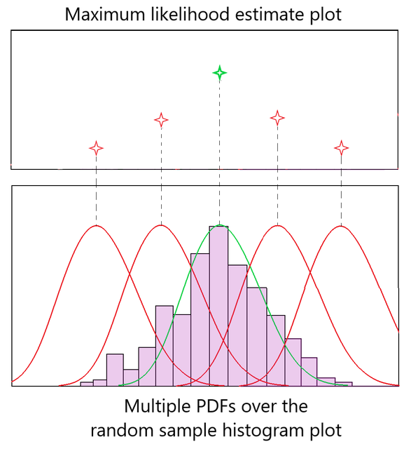
This figure perfectly illustrates the concept of MLE. We have a set of observed data points, shown as a histogram (bottom panel). We consider several candidate Gaussian distributions (the red and green curves), each defined by different parameters ($\mu$ and $\sigma^2$). For each candidate model, we can calculate how "likely" it is that it generated our data. The green curve fits the data best, and as the top panel shows, the parameter set corresponding to this curve yields the highest likelihood value. MLE is the principle of choosing those parameters.

The MLE Framework: From Products to Sums

Let's formalize this. Suppose we have a dataset of $n$ independent and identically distributed (i.i.d.) samples, $X = {x_{1}, x_{2}, ..., x_{n}}$ , drawn from a probability distribution $f (x ∣ θ)$ parameterized by $θ$ . Because the samples are independent, the joint probability of observing the entire dataset is the product of the individual probabilities:

P (X ∣ θ) = i = 1 \prod n f (x_{i} ∣ θ)

The likelihood function is defined using this expression, but viewed as a function of $θ$ :

L (θ ∣ X) = i = 1 \prod n f (x_{i} ∣ θ)

Our goal is to find the $θ$ that maximizes this function:

θ^_{M L E} = ar g θ max L (θ ∣ X)

In practice, working with a product of many small probabilities is mathematically cumbersome and can lead to numerical underflow issues in computation. A common and powerful technique is to instead maximize the logarithm of the likelihood. Since the logarithm is a strictly monotonically increasing function, the $θ$ that maximizes $L (θ)$ will also maximize $lo g (L (θ))$ . This log-likelihood function, often denoted $L (θ)$ or $LL (θ)$ , turns the product into a more manageable sum:

L (θ ∣ X) = lo g L (θ ∣ X) = lo g (i = 1 \prod n f (x_{i} ∣ θ)) = i = 1 \sum n lo g f (x_{i} ∣ θ)

Finding the maximum of this function is a standard calculus problem: we take the derivative with respect to $θ$ , set it to zero, and solve for $θ$ .

The following resource walks through this general framework and applies it to a concrete example.

[PDF] Maximum Likelihood Estimation

These lecture notes from Stanford's CS109 provide a concise mathematical summary of the MLE principle and a clear example.

Please read the first page of the document. Start with the introduction and the definition of the likelihood and log-likelihood functions. This formalizes the concepts we've just discussed. Then, follow the detailed derivation for the Bernoulli distribution. This shows the complete process: write the likelihood, take the log, sum the terms, and prepare to take the derivative. The result that the MLE for a Bernoulli parameter is the sample mean is a classic and intuitive first result.

MLE in Action: From Theory to Practice

Let's see how this works for a few key models.

Gaussian Distribution

What are the maximum likelihood estimates for the parameters $μ$ and $σ^{2}$ of a normal distribution? If we follow the MLE procedure—writing the log-likelihood for the Gaussian PDF and taking partial derivatives with respect to $μ$ and $σ^{2}$ —we arrive at highly intuitive results.

[PDF] Maximum Likelihood Estimation

Continuing in the same Stanford notes, let's look at the result for the Normal distribution.

Read the section titled "Normal MLE Estimation". You don't need to re-derive it yourself, but notice the results: \hat{\mu} = \frac{1}{n} \sum_{i=1}^{n} X_i (the sample mean) \hat{\sigma}^2 = \frac{1}{n} \sum_{i=1}^{n} (X_i - \hat{\mu})^2 (the sample variance) This confirms that the standard estimators for the mean and variance of a dataset can be derived directly from the MLE principle under the assumption of normality.

Connection to Linear Regression

Now for a more profound connection. The method of Ordinary Least Squares (OLS) for linear regression is typically introduced as an algorithm that minimizes the sum of the squared differences between predicted and actual values. But where does this objective come from? MLE provides the answer.

Let's assume our data is generated by a linear relationship with additive Gaussian noise. That is, $y_{i} = w^{T} x_{i} + ϵ_{i}$ , where the noise term $ϵ_{i}$ is drawn from a normal distribution with mean 0 and variance $σ^{2}$ , i.e., $ϵ_{i} \sim N (0, σ^{2})$ . This is equivalent to saying that the conditional probability of $y_{i}$ given $x_{i}$ is Gaussian:

p (y_{i} ∣ x_{i}, w, σ^{2}) = N (y_{i} ∣ w^{T} x_{i}, σ^{2})

If we now write down the log-likelihood for the entire dataset and seek to maximize it with respect to the weights $w$ , we will discover something remarkable.

[PDF] Machine Learning - MT 2016 3. Maximum Likelihood

These lecture slides from the University of Oxford provide a clear derivation linking MLE to least squares.

Please read through slides 7 to 12. Start on slide 7 to see the linear model with Gaussian noise assumption laid out. Follow the derivation on slides 9 and 10, which constructs the full likelihood and log-likelihood function. The key insight is on slide 11. Pay close attention to the log-likelihood expression. To maximize this function with respect to \mathbf{w}, we only need to consider the term that contains \mathbf{w}. All other terms are constants. Maximizing -\sum(y_i - \mathbf{w}^T\mathbf{x}_i)^2 is equivalent to minimizing \sum(y_i - \mathbf{w}^T\mathbf{x}_i)^2, which is precisely the least squares objective! Finally, slide 12 shows that this leads to the familiar closed-form solution for linear regression.

This is a critical insight: the principle of least squares is equivalent to maximum likelihood estimation under the assumption of Gaussian noise. This provides a powerful probabilistic justification for a widely used algorithm.

Furthermore, this framework is general. What if we assumed a different noise model? For instance, if we assume the noise follows a Laplace distribution (which has heavier tails than a Gaussian), the MLE principle leads to minimizing the sum of absolute differences, $\sum ∣ y_{i} - w^{T} x_{i} ∣$ , a method known to be more robust to outliers. The choice of probabilistic model for the data generating process directly dictates the form of the learning objective.

The Theoretical Power of MLE

Why is MLE so central to statistics and machine learning? Beyond its intuitive appeal and its ability to justify existing methods, estimators derived from MLE possess several highly desirable asymptotic properties (i.e., properties that emerge as the sample size grows large).

The most important theory in statistics | Maximum Likelihood

The "Very Normal" video provides a fantastic, clear summary of these theoretical guarantees.

Please watch the segment on the qualities of the MLE. It explains three key properties: Consistency: As the amount of data increases, the MLE gets closer and closer to the true parameter value. Asymptotic Normality: The distribution of the MLE approaches a Normal distribution as the sample size grows. This is the foundation for calculating confidence intervals and p-values for model parameters. Asymptotic Efficiency: The MLE achieves the lowest possible variance among a large class of unbiased estimators (it meets the Cramér–Rao lower bound). In essence, for large datasets, you can't find a more precise estimator.

These properties are the reason MLE is not just one method among many, but a cornerstone of statistical theory. It provides a recipe for generating estimators that are, in a very precise sense, the best possible.

Conclusion

In this lesson, we have established Maximum Likelihood Estimation as a general and powerful principle for fitting models to data.

Here are the key takeaways:

MLE as a Principle: MLE formalizes the intuitive idea of picking model parameters that make our observed data the most probable.
Log-Likelihood: We almost always work with the log-likelihood, which turns products into sums and simplifies the optimization process, a familiar pattern in algorithmic optimization.
Connecting Theory to Practice: MLE provides a deep, probabilistic justification for common objective functions. Assuming Gaussian noise leads to minimizing squared error (used in linear regression), while assuming Laplace noise leads to minimizing absolute error.
Theoretical Guarantees: MLE estimators are not just arbitrary; they possess strong theoretical properties like consistency, asymptotic normality, and efficiency, making them a gold standard in statistical inference.

We've now seen how to move from data description (PCA) to principled model fitting (MLE). In our next and final lesson of this module, we will introduce an even more general framework called Empirical Risk Minimization (ERM). You will see that MLE is a specific case of ERM, and this broader perspective will provide the final piece of our foundational mathematical toolkit before we dive into specific supervised learning algorithms.