Exploring VAE Latent Spaces

Welcome back! In our previous lesson, we constructed a Variational Autoencoder, moving from a simple deterministic compressor to a sophisticated probabilistic, generative model. You now understand the architecture, the objective function derived from the Evidence Lower Bound, and the clever reparameterization trick that makes it all trainable.

But building a model is only half the journey. A VAE, particularly its encoder, is a powerful feature engineering tool precisely because it learns a rich, structured, low-dimensional representation of your data. This representation is called the latent space, or the data manifold. This lesson is about demystifying that space. We will explore how to visualize it, probe its structure, and even perform "arithmetic" within it to understand and manipulate the abstract features the VAE has learned. This directly addresses your goal of mastering deep, complex feature generation methods by showing you how to verify and interpret the features a VAE creates.

Seeing the Manifold: Visualization

The latent space $Z$ of a VAE is typically high-dimensional (we've seen examples with 200 dimensions), which is impossible for us to perceive directly. To "see" the structure the VAE has learned, we must first project this high-dimensional space into a visualizable 2D or 3D space. Techniques like Principal Component Analysis (PCA), t-SNE, and Uniform Manifold Approximation and Projection (UMAP) are the tools for this job.

The goal of this projection is to arrange the data points in the lower-dimensional space such that their proximity reflects their similarity in the original high-dimensional latent space. A well-trained VAE, thanks to the KL divergence regularizer, produces a smooth and continuous latent space where similar inputs are mapped to nearby points. When we visualize this, we expect to see meaningful clusters and patterns emerge.

The following video provides an excellent intuition for what a latent space is and how dimensionality reduction helps us visualize it.

When this technique is applied, the results can be striking. The VAE effectively learns to organize the data according to its inherent semantic features. For instance, if we train a VAE on the MNIST handwritten digit dataset and then visualize its latent space with UMAP, we see distinct islands of points, where each island corresponds to a specific digit.

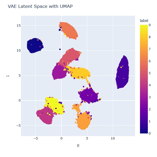
This clustering is direct evidence that the latent vectors are powerful features. A simple classifier (like k-Nearest Neighbors) operating in this latent space would perform vastly better than one operating on the raw, high-dimensional input data.

Exploring the Manifold: Traversal and Disentanglement

Visualization confirms that the latent space has structure. The next step is to explore it to understand what that structure means.

1. Latent Space Traversal and Interpolation

Because the VAE's latent space is continuous, we can "walk" from one point to another and observe the changes in the generated output. If we take the latent vectors for two different inputs, say $z_A$ and $z_B$, we can linearly interpolate between them: $z_{new}=(1-\alpha )z_A+\alpha z_B$. By feeding these interpolated vectors through the decoder for various values of $\alpha$ from 0 to 1, we can generate a smooth transition from the reconstruction of input A to input B. This demonstrates the model hasn't just memorized locations but has learned a smooth representation of the data's variations.

2. Disentanglement

A highly desirable property of a latent space is disentanglement. In a disentangled representation, single latent units are sensitive to changes in single generative factors, while being relatively invariant to changes in other factors. For example, in a VAE trained on faces, one ideal dimension might control the degree of smile, another the head pose, and a third the hair color, all independently.

Achieving perfect disentanglement is a major research area (models like $\beta$-VAE, which you saw briefly in the last lesson, aim for this). However, even standard VAEs often learn partially disentangled representations. We can test this by taking a latent vector, traversing along a single dimension (e.g., adding or subtracting a value from only the 5th component of the vector), and observing the effect on the decoded output.

Manipulating the Manifold: Latent Space Arithmetic

The most powerful demonstration of a meaningful latent space is the ability to perform arithmetic on latent vectors to manipulate the output semantically. This is a concept that truly feels like an "out of the box" technique.

The core idea is to identify directions in the latent space that correspond to specific attributes. The classic example involves adding a "smile" to a neutral face.

1. Find Attribute Vectors: Take all images labeled "smiling", pass them through the encoder to get their latent vectors $\{z_{smile}\}$, and compute the average vector, ${\vec{v}}_{smile}$. Do the same for "not smiling" images to get ${\vec{v}}_{neutral}$.
2. Calculate the Difference Vector: The vector representing the "smile" attribute is the difference: ${\vec{v}}_{smile\_attr}={\vec{v}}_{smile}-{\vec{v}}_{neutral}$.
3. Apply the Transformation: Take a new neutral face image, get its latent vector $z_{neutral\_new}$, and add the smile attribute vector to it: $z_{smiling\_new}=z_{neutral\_new}+\alpha \cdot {\vec{v}}_{smile\_attr}$, where $\alpha$ is a scaling factor.
4. Decode: Pass $z_{smiling\_new}$ through the decoder. The resulting image should be the original person, but now smiling.

The remarkable thing is that the VAE was trained in a purely unsupervised manner on the images themselves. The semantic attribute labels (like "smiling") are only used after training to discover the directions within the learned space.

Sebastian Raschka provides a fantastic, code-focused walkthrough of this exact process in PyTorch.

Quantitative Interpretation for Tabular Data

Visualizations and latent arithmetic are compelling, but they are qualitative and best suited for image data. For the tabular data common in finance and other domains you're interested in, we need a more rigorous, quantitative method of interpretation. How can we measure the influence of our original input features (e.g., 'annual_income', 'debt_to_income_ratio') on the latent space the VAE has learned?

A powerful technique for this is sensitivity analysis, which, given your background in mathematics, you can think of as a direct application of partial derivatives. The idea is to measure how sensitive the latent space parameters ($\mu$ and $\sigma$) are to small changes in each input feature.

A research paper focusing on VAEs for financial tabular data proposes exactly such a method. This is highly relevant to your goals.

The key takeaway from this paper is that we can compute a numerical score for each original feature that quantifies its contribution to the learned latent representation. If annual_income consistently produces large partial derivatives for the latent parameters, we know the VAE considers it a highly important feature for representing the data. Conversely, features with near-zero sensitivity and low interaction scores can potentially be removed, acting as a form of automated feature selection.

Conclusion

In this lesson, we have opened the "black box" of the Variational Autoencoder to examine what it learns. You now have a toolkit of both qualitative and quantitative methods to interpret the VAE's latent space.

Key Takeaways:

• Visualization: High-dimensional latent spaces can be projected into 2D/3D using methods like UMAP to visualize the learned data manifold, revealing clusters and structure.
• Qualitative Interpretation: Traversing the latent space allows for smooth interpolation between data points. In disentangled representations, individual latent dimensions control specific, meaningful data attributes.
• Latent Space Arithmetic: We can perform vector operations on latent embeddings to semantically manipulate the data output, proving the space has captured high-level concepts.
• Quantitative Interpretation: For tabular data, sensitivity analysis provides a rigorous method to measure the importance of each input feature by calculating the partial derivatives of the latent parameters with respect to the inputs.

Interview Alert
Question: "You've used a VAE to learn features from tabular data. How would you convince a non-technical stakeholder that these abstract, learned features are meaningful and trustworthy?"

Your Answer: You would explain that you can interpret these features in several ways. First, you can use visualization techniques like UMAP to show that the VAE has learned to group similar data points (e.g., customers who churn vs. those who don't) into distinct clusters in its latent space. More powerfully, for tabular data, you can use quantitative methods like sensitivity analysis. This allows you to produce a feature importance plot, demonstrating precisely which original input features (like 'customer tenure' or 'monthly charges') have the biggest impact on the VAE's learned representation. This bridges the gap between the abstract latent features and the concrete, understandable business inputs.

Preview of the Next Lesson:
We have now seen how autoencoders and VAEs can be used for unsupervised feature generation. Next, we will explore a different deep learning architecture designed specifically for tabular data that incorporates interpretability directly into its design: TabNet. You will learn how its use of sequential attention allows for instance-wise feature selection, providing a different but equally powerful approach to feature engineering and interpretation.