TabNet: Sequential Attention for Feature Selection

Welcome to the next step in our journey into deep learning for tabular data. In our last lesson, we explored Variational Autoencoders (VAEs), an unsupervised method for learning a rich, continuous latent representation of your data. You saw how we could interpret this latent space both visually and quantitatively to understand the abstract features the model had generated.

Today, we shift from unsupervised feature generation to supervised feature selection, but with a unique deep learning twist. We will delve into TabNet, an architecture from Google AI that has challenged the dominance of gradient boosting models like XGBoost on tabular data. Instead of creating new, abstract features like a VAE, TabNet learns to intelligently select the most salient original features for each individual prediction. This powerful concept, known as instance-wise feature selection, offers both high performance and a remarkable degree of interpretability, directly addressing your goal of understanding complex, "out of the box" methods.

By the end of this lesson, you will understand the mechanics of TabNet's sequential attention mechanism and be able to implement the model to leverage its unique capabilities for feature selection and explanation.

The Motivation Behind TabNet

For years, deep learning models have reigned supreme in domains like computer vision and NLP. However, on structured, tabular data, tree-based ensembles such as XGBoost and LightGBM have consistently held the top spot. TabNet was designed to bridge this gap. It's a novel deep learning architecture that attempts to import principles from decision trees into a neural network framework.

The core idea is to process features sequentially, in steps, much like how a decision tree makes a series of splits. At each step, the model decides which features to focus on, effectively learning a feature selection policy that is tailored to each individual data sample.

The Architecture: A Sequence of Decisions

TabNet processes information in multiple decision steps. In each step, it performs two main actions:

1. It selects a subset of features using an Attentive transformer.
2. It processes these selected features using a Feature transformer to produce part of the final output.

The final prediction is an aggregation of the outputs from all steps.

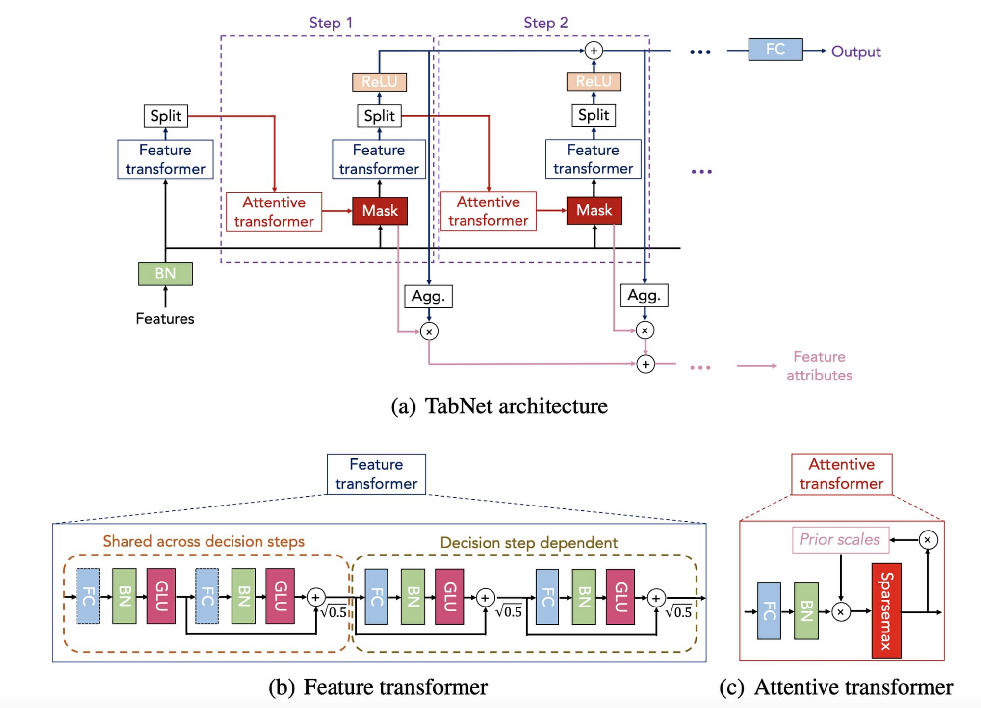
This sequential process is powerful because it allows the model to reason about features in a structured way. For example, in Step 1, it might use 'age' and 'occupation' to make a broad determination. Then, in Step 2, conditioned on that information, it might focus on a completely different set of features like 'hours-per-week' and 'capital-gain' to refine its prediction.

At the Heart of TabNet: The Transformers

Let's break down the two key components.

1. The Attentive Transformer and Instance-Wise Selection

The job of the attentive transformer is to create a learnable mask, M[i], at each step i. This mask determines which features to pay attention to. Since your experience lies in computer engineering and signal processing, you can think of this mask as a filter that is dynamically designed for each input signal (each data row).

Two innovations make this possible:

• Sparsemax Normalization: Instead of a standard softmax function which assigns some probability to all features, the attentive transformer uses Sparsemax. Sparsemax pushes the probabilities for less relevant features to exactly zero, creating a sparse mask that performs "hard" feature selection. This is critical for both performance and interpretability.

• Prior Scaling: To encourage the model to use different features at different steps, the attentive transformer uses a "prior scale" term, P[i]. This term tracks which features have been used in previous steps. Specifically, P[i] = (γ - M[i-1]) * P[i-1], where γ is a relaxation parameter. If a feature was heavily used in the previous mask M[i-1], its corresponding value in P[i] will be small, discouraging its reuse in the current step. This forces the model to explore a diverse set of features throughout its decision-making process.

2. The Feature Transformer

Once the mask is applied to the input features, the selected features are passed to the Feature Transformer. This module's job is to process the information and produce two outputs: one that contributes to the final prediction, and another that is passed to the next step's attentive transformer.

This block is essentially a series of fully-connected layers with a special activation function and residual connections.

• Gated Linear Units (GLU): Instead of a standard ReLU, the feature transformer uses GLUs. A GLU block applies a sigmoid gate to the input, controlling what information is allowed to flow through the network. This gating mechanism, similar in spirit to those in LSTMs or GRUs that you may have encountered in NLP, allows for more complex, dynamic routing of information.

• Shared and Independent Blocks: For parameter efficiency, some GLU blocks within the feature transformer are shared across all decision steps, learning transformations that are broadly useful. Other blocks are independent, allowing each step to learn step-specific transformations.

The article "Implementing TabNet in PyTorch" provides clear, concise code snippets that demystify these components.

The Payoff: Instance-Wise Interpretability

The true power of TabNet, especially compared to other "black box" deep learning models, is its built-in interpretability. The masks M[i] generated by the attentive transformer at each step are not just an internal mechanism; they are a direct output that explains the model's reasoning.

By aggregating the masks across all steps for a single prediction, we can create a feature importance plot that is specific to that one data point. This is instance-wise explainability.

The image below shows this in action on two synthetic datasets.

• Syn2: The output depends on a fixed set of features (X3 to X6).
• Syn4: The output depends on features X1-X2 OR X3-X6, depending on the value of another feature, X11. This requires instance-wise selection.

Notice how for Syn4, the attention patterns (M[1], M[2], etc.) are different for different samples (rows). This is TabNet learning to apply different rules and focus on different features for each case, just as you would when debugging different failing test cases in a complex software system.

Implementing TabNet with pytorch-tabnet

While understanding the architecture is key, you don't need to implement it from scratch every time. The pytorch-tabnet library provides a scikit-learn compatible interface that makes using TabNet incredibly simple.

The creator of the library gives an excellent hands-on demonstration.

Conclusion

In this lesson, you have explored TabNet, a deep learning architecture that brings a novel approach to tabular data by incorporating principles from decision trees. You've moved beyond the feature generation of VAEs to the intelligent, instance-wise feature selection of TabNet.

Key Takeaways:

• Hybrid Approach: TabNet combines the end-to-end training and representation learning power of deep learning with the feature selection capabilities of tree-based models.
• Sequential Attention: The model processes data in steps, using an Attentive Transformer with Sparsemax to select a sparse set of the most relevant features at each step.
• Instance-Wise Selection: The feature selection is not global; it is tailored to each individual data sample, allowing the model to learn more complex decision rules.
• Built-in Interpretability: The attention masks used for feature selection double as a direct explanation of the model's reasoning for each prediction.
• Practical Implementation: Libraries like pytorch-tabnet make it straightforward to apply this powerful architecture using a familiar API.

Interview Alert
Question: "When would you choose TabNet over a model like XGBoost for a tabular data problem?"

Your Answer: "While XGBoost is an incredibly strong and often faster baseline, I would consider TabNet in several scenarios. First, if the problem requires instance-wise interpretability, TabNet provides this natively through its attention masks, which is more direct than post-hoc explanation methods like SHAP on XGBoost. Second, in a multimodal setting where I need to combine tabular data with images or text, TabNet's deep learning nature allows it to be integrated into a larger, end-to-end trainable model. Finally, if there's potential for self-supervised pre-training on a large unlabeled tabular dataset, TabNet can be pre-trained to learn meaningful representations, which can then be fine-tuned on a smaller labeled dataset, a strategy not available to XGBoost."

Preview of the Next Lesson:
We have now seen how autoencoders can generate new features and how TabNet can select existing ones. In our next lesson, we will explore another powerful technique borrowed from the computer vision world: 1D Convolutional Neural Networks (CNNs). You will learn how to apply 1D convolutions to tabular data to automatically learn features based on local patterns and interactions between adjacent features, which is particularly effective when your features have a natural sequence or spatial ordering.