Autoencoders for Tabular Data: Feature Extraction and Dimensionality Reduction

Welcome to your first lesson in the module on Deep Learning for Tabular Feature Generation. Your goal to explore "out of the box" and complex feature engineering methods aligns perfectly with this module's focus. We'll be moving beyond traditional, handcrafted features and delving into how neural networks can learn powerful, dense feature representations directly from data.

In this lesson, you will learn to implement an autoencoder for unsupervised feature extraction and dimensionality reduction on tabular data. This is a foundational technique that serves as a launchpad for many of the more advanced deep learning approaches we'll cover. We will explore the core concepts behind autoencoders, build one from scratch using PyTorch, and evaluate the utility of the features it generates.

The "What" and "Why" of Autoencoders

In many real-world scenarios, you'll encounter datasets with a large number of features. These features might be redundant, correlated, or noisy. Manually sifting through them to engineer new, more informative features is both an art and a science, but it can be time-consuming and requires significant domain expertise.

Autoencoders offer an alternative: a neural network-based approach to learn a compressed, lower-dimensional representation of your data in a completely unsupervised manner. This means the model learns the underlying structure of the data without needing any labels.

To start, let's build a strong conceptual foundation. The following short, animated video provides an excellent overview of the autoencoder's architecture and training process.

As the video illustrates, an autoencoder consists of two main parts:

1. The Encoder: This part of the network takes the high-dimensional input data and compresses it into a low-dimensional representation. This compressed representation is often called the latent space or bottleneck.
2. The Decoder: This part takes the compressed representation from the bottleneck and attempts to reconstruct the original, high-dimensional input data.

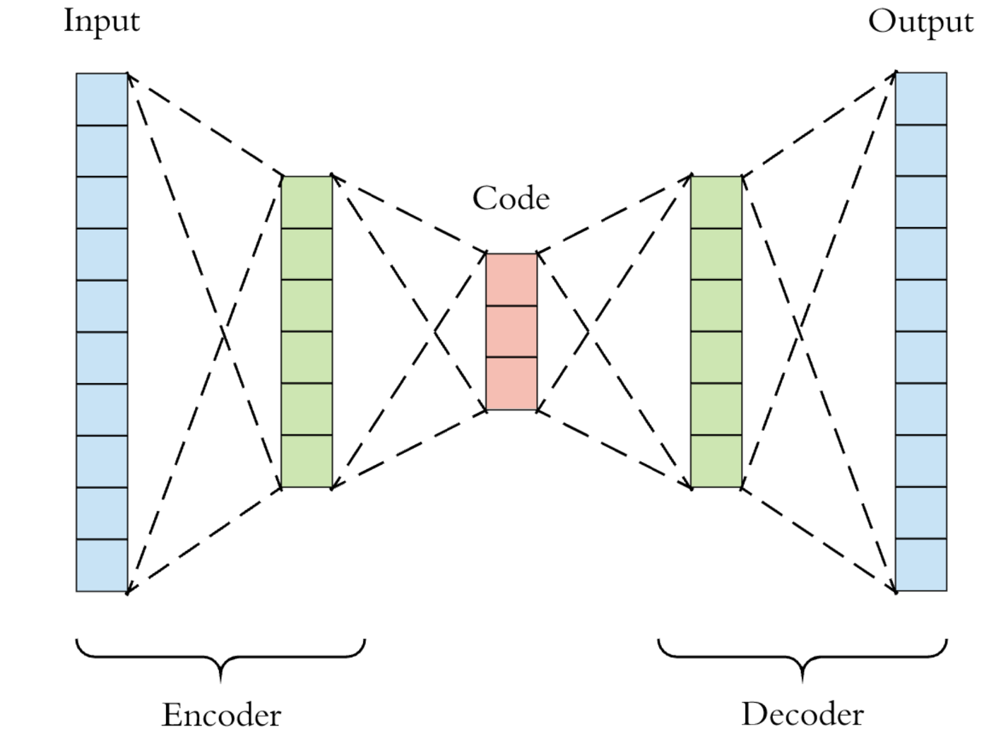
The magic happens during training. The network's sole objective is to make the output as identical to the input as possible. By forcing the data to pass through the narrow bottleneck, the encoder must learn to capture the most essential and salient information, effectively discarding noise and redundancy. This learned mapping—from the input to the latent space—is our feature extractor.

A Hands-On Implementation in PyTorch

Now, let's translate this theory into practice. Given your proficiency with PyTorch, we can move directly to a practical example. We'll use a detailed hands-on guide that walks through building an autoencoder for synthetic tabular data.

The following reading provides all the code and explanations for the entire workflow, from data preparation to evaluating the extracted features.

The choice of the final activation function in the decoder is critical and directly depends on how you scale your input data. The hands-on guide uses MinMaxScaler (scaling to [0, 1]) and thus uses a Sigmoid function. This is a common pattern. For a different perspective, you might find this short clip from a tutorial on image autoencoders helpful.

From Unsupervised Learning to Supervised Tasks

You've now seen how to train an autoencoder and use its encoder to generate new features. The ultimate test of these features is their performance on a downstream supervised task, such as classification or regression.

The process typically looks like this:

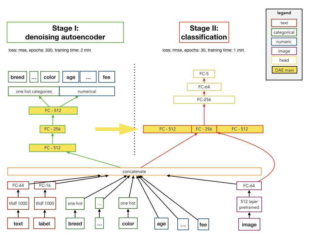
1. Stage I (Unsupervised Pre-training): Train an autoencoder on your entire dataset (or a large, unlabeled portion of it) to learn a robust, low-dimensional representation.
2. Stage II (Supervised Fine-tuning/Training): Use the trained encoder as a fixed feature extractor. Feed your data through the encoder to get the latent representations, and then train a simpler, separate model (like Logistic Regression, Gradient Boosting, or a small neural network) on these new features using your labeled data.

The diagram below illustrates this two-stage approach. While it specifically shows a denoising autoencoder (a variant that learns to reconstruct clean data from intentionally corrupted inputs), the overall workflow is the same.

Conclusion

In this lesson, you've taken the first step into using deep learning for feature engineering on tabular data. You've learned how autoencoders can perform non-linear dimensionality reduction in an unsupervised fashion, and you've walked through a complete implementation in PyTorch.

Key Takeaways:

• Autoencoders learn a compressed representation of data by trying to reconstruct their own input.
• The encoder part of a trained autoencoder serves as a powerful, non-linear feature extractor.
• The dimensionality of the latent space (latent_dim) is a critical hyperparameter that controls the trade-off between information compression and reconstruction quality.
• Model design choices, such as the decoder's output activation function, must be consistent with the data preprocessing steps.

Interview Alert
In a system design interview, you might be asked how to handle a dataset with hundreds of potentially correlated numerical features. Proposing an autoencoder as a non-linear dimensionality reduction technique is a strong, modern answer. You should be prepared to discuss the trade-offs: the computational cost of training, the potential loss of interpretability (the new features are abstract), and the need to tune hyperparameters like the latent space dimension.

Preview of the Next Lesson:
We've explored the basic autoencoder, which maps each input to a single, deterministic point in the latent space. In the next lesson, we will explore its probabilistic cousin: the Variational Autoencoder (VAE). A VAE learns to map each input to a distribution in the latent space, which not only yields powerful features but also turns the decoder into a generative model capable of creating new, synthetic data samples. This opens up a whole new range of advanced applications.