Autoencoders: Dimension Reduction & Reconstruction

Hello! Welcome to the next module in your AI Engineering course.

In our previous lessons, we mastered the art of building, fine-tuning, and evaluating discriminative models, like the Transformer-based classifiers you worked with. These models are experts at learning boundaries between different classes of data. Now, we are pivoting to a new and exciting domain: generative modeling. Instead of just classifying data, our goal will be to learn the underlying distribution of the data itself, enabling us to create entirely new samples.

This lesson marks our first step into this world. We will explore the architecture and purpose of a standard autoencoder. You will learn how these neural networks are designed for dimensionality reduction and data reconstruction, which serves as a crucial conceptual foundation for the more advanced generative models we'll tackle next, such as Variational Autoencoders (VAEs) and Generative Adversarial Networks (GANs).

1. The Architecture of an Autoencoder

At its core, an autoencoder is a type of neural network trained in an unsupervised manner. Its goal is surprisingly simple: to reconstruct its own input. While this might sound trivial, the network's architecture forces it to learn something profound about the data in the process.

To start, let's get a high-level animated overview of what an autoencoder is and its fundamental components.

As the video explained, a standard autoencoder is composed of three main parts:

1. The Encoder: This part of the network takes the high-dimensional input data and compresses it into a lower-dimensional representation. It learns to extract the most salient features.
2. The Bottleneck (or Latent Space): This is the central, most compressed layer of the network. The output of the encoder, often called the "code" or "encoding," resides here. Its dimensionality is a critical hyperparameter, defining how much the data is compressed.
3. The Decoder: This part takes the compressed code from the bottleneck and attempts to reconstruct the original high-dimensional input data from it.

The entire structure is often symmetric, forming an hourglass shape where the input and output layers have the same number of neurons.

2. The Purpose: Reconstruction and Dimensionality Reduction

Why would we train a network to just copy its input? The magic lies in the bottleneck. Because the latent space has a smaller dimension than the input, the network cannot simply memorize and pass through the data. It is forced to learn an efficient, compressed representation that captures the essential information needed for reconstruction. This constraint is what makes autoencoders powerful tools for dimensionality reduction.

How an Autoencoder Learns

The network is trained by minimizing the reconstruction loss, which is the difference between the original input and the reconstructed output. For data like images, a common loss function is the Mean Squared Error (MSE), which calculates the average squared difference between the pixel values of the original and reconstructed images.

Here, $x$ is the original input and $x^{\prime }$ is the reconstructed output. Through backpropagation, the network adjusts its weights to make $x^{\prime }$ as close to $x$ as possible.

Connection to Principal Component Analysis (PCA)

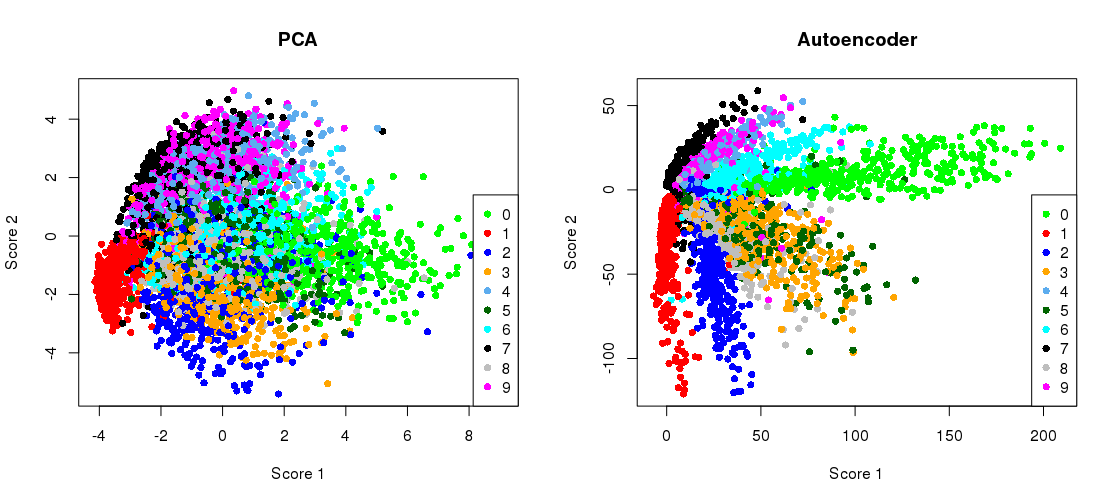
Given your background in classic machine learning, you're likely familiar with PCA as a technique for dimensionality reduction. There's a deep connection here: a simple autoencoder with a single hidden layer and linear activation functions is mathematically equivalent to PCA. It learns to project the data onto a lower-dimensional subspace that captures the principal components.

However, the real power of autoencoders comes from their ability to be non-linear.

By adding non-linear activation functions (like ReLU, Tanh, or Sigmoid) to the encoder and decoder, autoencoders can learn much more complex, non-linear manifolds in the data. This allows them to create more powerful and flexible embeddings than PCA.

To solidify this point, this brief document provides a more formal look at the relationship between PCA and autoencoders.

The practical result is that an autoencoder's latent space can often be more "organized" and useful than the space produced by PCA, with clearer separation between different classes of data.

3. A Glimpse into the Code

You've now used PyTorch to build complex models like CNNs and LSTMs. Building a simple autoencoder is refreshingly straightforward. While we won't implement and train one today, looking at the code structure helps make the architecture concrete.

We can define a shallow autoencoder with a single hidden layer using nn.Sequential, just as you've seen before.

As you saw in the resource, the structure is very clear. For an MNIST image (28x28 = 784 pixels) and a 32-dimensional latent space, the model would look like this:

import torch.nn as nn

input_size = 784
encoding_size = 32

model = nn.Sequential(



    # Encoder
    nn.Linear(input_size, encoding_size),
    nn.ReLU(),
    



    # Decoder
    nn.Linear(encoding_size, input_size),
    nn.Sigmoid() 
)

print(model)

Output:

Sequential(
  (0): Linear(in_features=784, out_features=32, bias=True)
  (1): ReLU()
  (2): Linear(in_features=32, out_features=784, bias=True)
  (3): Sigmoid()
)

Here's the breakdown:

• The first nn.Linear layer compresses the 784 input pixels down to the encoding_size of 32. This, along with its activation, is the encoder.
• The second nn.Linear layer expands the 32-dimensional code back to the original 784 dimensions. This is the decoder.
• The nn.Sigmoid activation in the final layer is a common choice for image reconstruction when pixel values are normalized between 0 and 1, as it constrains the output to be in that same range.

Conclusion

In this lesson, you've learned the fundamentals of standard autoencoders. They are a simple yet powerful unsupervised learning tool that lays the groundwork for more complex generative models.

Key Takeaways:

• Architecture: Autoencoders consist of an encoder, a bottleneck (latent space), and a decoder. The network is trained to reconstruct its input.
• Purpose: The primary purposes are unsupervised data reconstruction and dimensionality reduction.
• Learning Mechanism: The bottleneck forces the network to learn a compressed, meaningful representation of the data instead of just copying it.
• Advantage over PCA: By using non-linear activation functions, autoencoders can learn complex, non-linear relationships in data, making them more powerful for dimensionality reduction than linear methods like PCA.

Preview of the Next Lesson

Autoencoders are great at learning compressed representations and reconstructing data. But what if we want to generate new data that looks like our training data, but isn't just a reconstruction? A standard autoencoder's latent space isn't structured enough for that. If we pick a random point in the latent space and pass it to the decoder, the output is often meaningless.

In our next lesson, we will introduce the Variational Autoencoder (VAE). You'll learn how VAEs modify the autoencoder architecture to learn a smooth, probabilistic latent space that we can intelligently sample from to generate novel, high-quality data.