Understanding VAE Architecture and Objectives

Hello! Welcome back to our module on Generative Models.

In our last lesson, we explored the standard autoencoder. We learned that while it's excellent for compressing data into a latent space and reconstructing it, its primary limitation is a disorganized latent space. If you were to pick a random point from that space and feed it to the decoder, you'd likely get a meaningless, noisy output. This makes standard autoencoders unsuitable for generating new, coherent data.

Today, we'll address this exact problem by diving into the Variational Autoencoder (VAE). This lesson will explain the VAE's unique architecture and its clever training objective. You will learn how VAEs impose a structure on the latent space, transforming it from a simple codebook into a rich, continuous landscape from which we can generate novel data.

1. From a Point to a Distribution: The VAE's Core Idea

The fundamental shift from a standard autoencoder to a VAE is in how we think about the latent space. A standard autoencoder maps an input to a single point in the latent space. A VAE, on the other hand, maps an input to a probability distribution.

This means the encoder's job is not to output a single vector of coordinates z, but to describe the parameters of a distribution from which we can then sample a z. Typically, this distribution is a simple Gaussian.

This video from Deepia provides an excellent animated overview of this core concept.

The VAE Architecture

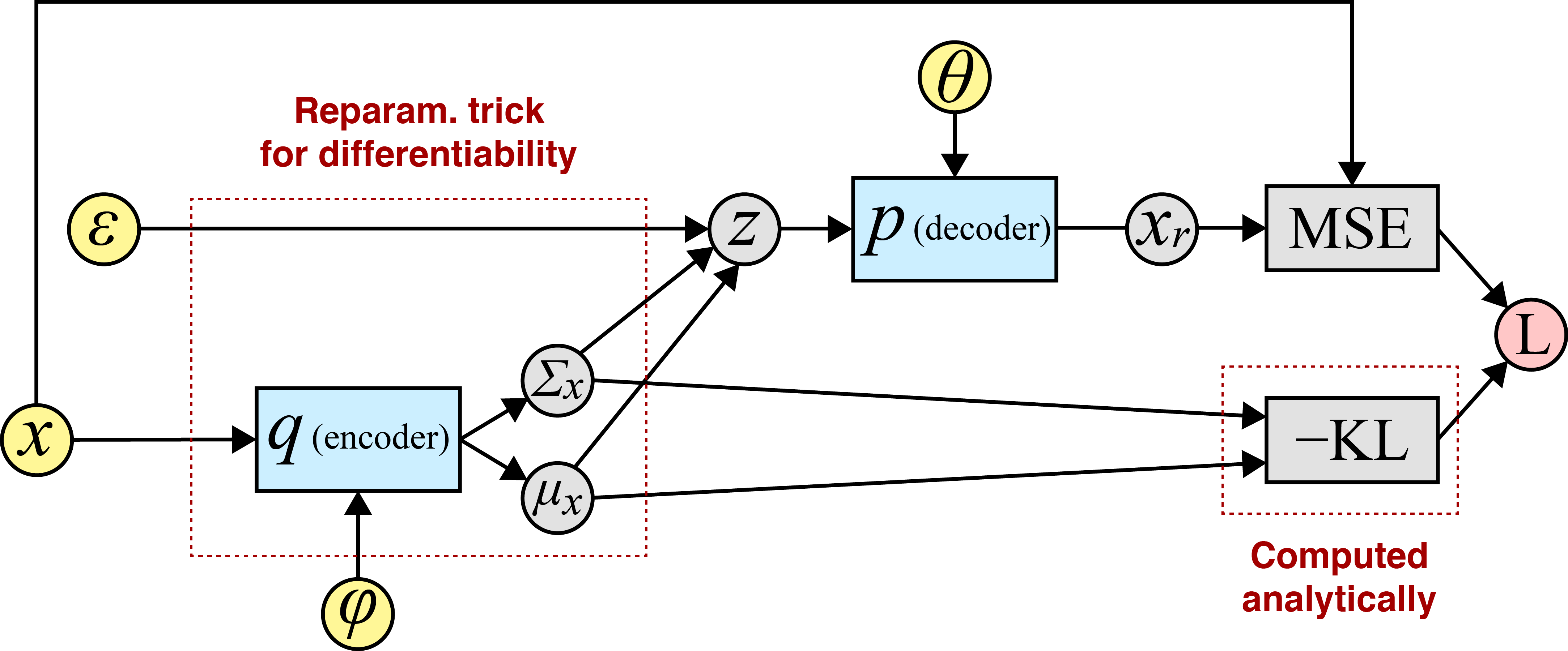
As the video explained, the VAE architecture modifies the encoder:

1. Encoder (q(z|x)): Instead of one output vector, the encoder produces two: a mean vector (μ) and a log-variance vector (log(σ²)). These two vectors parameterize a Gaussian distribution in the latent space for the given input x. We use log-variance for numerical stability, as variance must always be positive.
2. Sampling: We then sample a latent vector z from this distribution: z ~ N(μ, σ²). This step introduces controlled randomness.
3. Decoder (p(x|z)): The decoder takes the sampled latent vector z and reconstructs the original input x, just like in a standard autoencoder.

This process is elegantly illustrated in the diagram below.

2. The VAE Objective: Maximizing the Evidence Lower Bound (ELBO)

How do we train such a network? The goal is to create a model that accurately represents the data distribution. Mathematically, this means maximizing the log-likelihood of our data, log p(x). However, for the VAE model, this quantity is intractable to compute directly because it requires integrating over all possible latent variables z.

To overcome this, VAEs use a technique from variational inference. Instead of maximizing log p(x) directly, we maximize a tractable lower bound on it, called the Evidence Lower Bound (ELBO).

The VAE's loss function is simply the negative of the ELBO. Maximizing the ELBO is the same as minimizing the negative ELBO. With some derivation (which we'll look at optionally), the ELBO can be expressed in a very intuitive form with two key components.

So, the loss we want to minimize is:

Let's break down these two parts:

1. Reconstruction Loss:

   • This is the term - \mathbb{E}_{z \sim q(z|x)}[\log p(x|z)].
   • It measures the expected negative log-likelihood of the original input x given the sampled latent vector z.
   • In simpler terms, it's the error between the original input and the output from the decoder. For images, this often simplifies to the Mean Squared Error (MSE), just as in a standard autoencoder. This term pushes the model to learn to reconstruct the input faithfully.

2. Regularization (KL Divergence):

   • This is the term D_{KL}(q(z|x) || p(z)).
   • The Kullback-Leibler (KL) divergence is a measure of how one probability distribution differs from a second, reference distribution.
   • Here, it measures the "distance" between the distribution produced by our encoder, q(z|x), and a fixed prior distribution we choose for the latent space, p(z).
   • This prior p(z) is almost always chosen to be a standard normal distribution: N(0, I).
   • This term acts as a regularizer. It forces the encoder to learn distributions that are close to the standard normal distribution. This prevents the encoder from "cheating" by creating very specific, far-apart distributions to achieve perfect reconstruction. It encourages all encoded distributions to cluster around the origin, creating a continuous and well-organized latent space.

The training process is a balancing act between these two loss terms. The reconstruction loss encourages uniqueness and detail, while the KL divergence encourages similarity and structure.

To formalize this concept, the following resource provides a clear textual breakdown of the VAE loss function.

Optional: The Mathematical Derivation of ELBO

Given your interest in the mathematical foundations, you might want to see how the ELBO is derived. This is not essential for a practical understanding but provides the theoretical underpinning. The derivation uses Jensen's inequality, which you may remember from your statistics courses.

The following text provides a step-by-step derivation.

3. The Reparameterization Trick: Making Sampling Differentiable

There's one final, crucial piece of the puzzle. To train a neural network, we need to use backpropagation to calculate gradients. But our VAE architecture includes a sampling step: z is randomly drawn from N(μ, σ²). This is a stochastic (random) node, and we cannot pass gradients through it.

So, how do we train the encoder? The solution is a clever technique called the reparameterization trick.

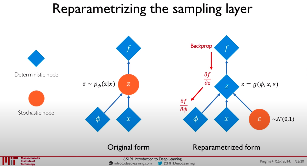
The trick reframes the sampling process. Instead of sampling z directly from N(μ, σ²), we do the following:

1. Sample a random noise vector ε from a standard normal distribution, ε ~ N(0, I). This random source is outside our main network graph.
2. Compute z deterministically as: z = μ + σ * ε.

This simple change makes the entire path from the encoder's parameters to the final loss function differentiable. We can now backpropagate the gradients from the loss all the way back to the weights of the encoder.

This last video segment clearly explains and animates this essential trick.

Conclusion

In this lesson, you've moved from the concept of a standard autoencoder to the more powerful and generative Variational Autoencoder. You now understand the key architectural and theoretical changes that enable VAEs to learn a structured latent space suitable for generating new data.

Key Takeaways:

• Probabilistic Encoding: VAEs encode an input x into a probability distribution (typically a Gaussian defined by a mean μ and variance σ²) in the latent space, rather than a single point.
• The ELBO Objective: VAEs are trained by minimizing the negative Evidence Lower Bound (ELBO), which consists of two terms:
  • A reconstruction loss that ensures the decoder can accurately reconstruct the input from a latent sample.
  • A KL divergence term that regularizes the latent space, forcing the learned distributions to be close to a standard normal prior N(0, I). This creates a continuous and organized space.
• The Reparameterization Trick: This essential technique makes the stochastic sampling process differentiable by moving the source of randomness outside the main computation graph, enabling end-to-end training with backpropagation.

Preview of the Next Lesson

Now that you have a solid grasp of the theory behind VAEs, it's time to put it into practice. In the next lesson, you will implement and train a VAE from scratch on an image dataset using PyTorch. You'll see how the concepts of the probabilistic encoder, the ELBO loss function, and the reparameterization trick translate directly into code.