Understanding GANs: Generator, Discriminator, and Training

Hello! Welcome to our next lesson in the "Foundations of Generative Models" module.

In the previous lesson, we explored how to generate new images using a trained Variational Autoencoder (VAE). We saw that by enforcing a smooth, continuous structure on the latent space, we could sample from it to create novel data. However, as we noted, VAE-generated images often have a characteristic blurriness.

Today, we will dive into a different and highly influential class of generative models that addresses this issue: Generative Adversarial Networks (GANs). Instead of a single network, GANs use two networks that compete against each other, leading to remarkably sharp and realistic results.

Our learning objective for this lesson is to explain the generator-discriminator framework of a Generative Adversarial Network (GAN) and its training objective. We will cover the roles of the two networks, the game-like dynamic they engage in, and the mathematical function that governs their training.

1. The Adversarial Framework: A Game of Cat and Mouse

At the heart of a GAN is a pair of neural networks locked in a competitive game. This adversarial relationship is a powerful mechanism for learning. A common and very effective analogy is that of an art forger and an art critic.

To get a clear picture of this dynamic, let's watch a short introductory video.

As the video illustrates, a GAN consists of two main components:

1. The Generator (G): Its job is to create synthetic data that is indistinguishable from real data. It takes a random noise vector z (sampled from a latent space, much like with VAEs) as input and outputs a data sample (e.g., an image).
2. The Discriminator (D): Its job is to act as a binary classifier. It takes a data sample (either a real one from the training set or a fake one from the generator) and outputs a probability indicating whether the sample is real or fake.

The two networks are trained together. The generator tries to get better at fooling the discriminator, while the discriminator tries to get better at catching the generator's fakes. This "cat and mouse" game forces the generator to produce increasingly realistic data.

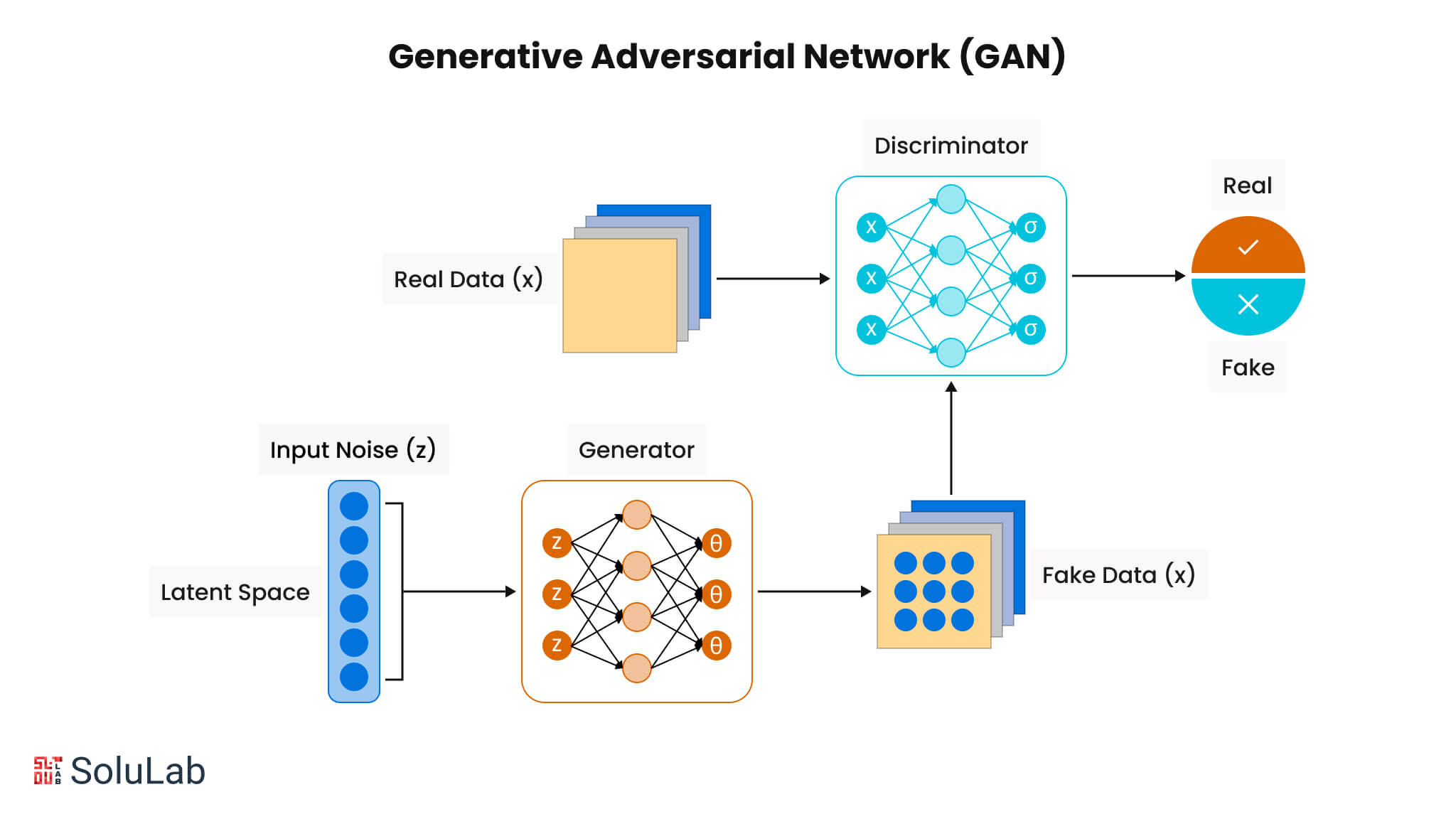
To understand the data flow and the underlying probability distributions, let's watch another short segment.

2. The Training Objective: A Minimax Game

Now that you understand the framework, let's formalize the training objective. The adversarial training process is mathematically defined as a minimax game between the generator and the discriminator. This is described by a single value function, V(D, G).

The goal is to find the parameters for the generator and discriminator that represent a solution to this game. The overall objective function is:

This equation might seem complex, but it's built on a concept you're familiar with: Binary Cross-Entropy (BCE) loss. Since the discriminator is a binary classifier (real vs. fake), its loss is essentially a BCE loss.

Let's break down the value function:

• The Discriminator's Goal (max_D V(D, G)): The discriminator wants to maximize the value function.

  • For the first term, ${\mathbb{E}}_{x\sim p_{\text{data}}(x)}[\log D(x)]$, when it receives a real sample $x$, it wants to make its output $D(x)$ as close to 1 (real) as possible. This maximizes $\log D(x)$.
  • For the second term, ${\mathbb{E}}_{z\sim p_z(z)}[\log (1-D(G(z)))]$, when it receives a fake sample $G(z)$, it wants to make its output $D(G(z))$ as close to 0 (fake) as possible. This makes $1-D(G(z))$ close to 1, which in turn maximizes $\log (1-D(G(z)))$.
  • In short, the discriminator maximizes the value function by correctly classifying real and fake samples.

• The Generator's Goal (min_G V(D, G)): The generator wants to minimize the value function.

  • The generator has no control over the first term, $\log D(x)$, as it doesn't produce real data.
  • It can only influence the second term, $\log (1-D(G(z)))$. To minimize this value (i.e., make it a large negative number), the generator must produce fake samples $G(z)$ that the discriminator classifies as real, making $D(G(z))$ close to 1. When $D(G(z))$ is close to 1, $1-D(G(z))$ is close to 0, and $\log (1-D(G(z)))$ approaches $-\infty$.
  • In short, the generator minimizes the value function by fooling the discriminator.

The following video provides a step-by-step derivation of this value function from the familiar BCE loss, which will solidify your understanding.

3. The Training Loop and Convergence

In practice, we cannot solve the minimax problem all at once. Instead, we use an iterative, alternating training process:

1. Train the Discriminator: We freeze the generator's weights and train the discriminator for one or more steps. We feed it a batch of real images (labeled as 1) and a batch of fake images generated by the current generator (labeled as 0). The discriminator updates its weights via gradient ascent to maximize the value function (or equivalently, minimize its BCE loss).
2. Train the Generator: We freeze the discriminator's weights and train the generator for one step. We generate a new batch of fake images and pass them through the discriminator. The generator then updates its weights via gradient descent to minimize the value function—specifically, to make the discriminator classify its output as real (label 1).

This cycle repeats, with both networks improving in turn.

What does convergence look like?

The training process ideally reaches a point of equilibrium where:

• The generator's output distribution, $p_g$, has converged to the real data distribution, $p_{\text{data}}$. The generated samples are indistinguishable from real ones.
• The discriminator is no longer able to tell the difference between real and fake samples. For any input, it outputs a probability of 0.5.

Given your mathematical background, you might appreciate the theoretical guarantee behind this. It can be shown that at the optimal point of this minimax game, the value function is minimized precisely when the generator's distribution is identical to the real data distribution. This minimization is equivalent to minimizing the Jensen-Shannon (JS) divergence between the two distributions.

Conclusion

In this lesson, we have established the theoretical foundation of Generative Adversarial Networks. You are now equipped with the core concepts needed to understand how GANs work.

Key Takeaways:

• Adversarial Framework: GANs consist of a Generator (the forger) that creates synthetic data from noise and a Discriminator (the critic) that tries to distinguish real data from fake data.
• Minimax Game: The training is framed as a game where the discriminator tries to maximize a value function (by being a good critic), and the generator tries to minimize it (by being a good forger).
• Value Function: The GAN objective function is derived from the Binary Cross-Entropy loss and measures how well the discriminator can separate real from fake, and how well the generator can fool the discriminator.
• Convergence: The ideal outcome of training is reaching an equilibrium where the generator produces data so realistic that the discriminator can no longer tell the difference, outputting a 50% probability for any sample.

Preview of the Next Lesson

With this theoretical grounding, we are ready to move to implementation. In the next lesson, you will implement the generator and discriminator networks for a simple image GAN in PyTorch. We will define the network architectures and write the alternating training loop to bring this powerful generative model to life.