Introduction to Singular Value Decomposition (SVD)

Hello! Welcome to your next lesson in our journey through the mathematical foundations of AI.

Introduction

In our last lesson, we saw how Principal Component Analysis (PCA) can be used for dimensionality reduction. We concluded with a preview of a more general and numerically robust method for this task: the Singular Value Decomposition (SVD). We briefly mentioned that the SVD of the data matrix itself contains all the information needed for PCA, bypassing the explicit formation of the covariance matrix.

Today, we will formally define the Singular Value Decomposition. Our learning outcome is to define the SVD and the properties of its constituent matrices (U, Σ, V). Unlike eigendecomposition, which is limited to certain square matrices, the SVD exists for any rectangular matrix. This universality makes it one of the most fundamental and powerful matrix decompositions in linear algebra and data science.

We will derive the SVD from first principles, building upon your understanding of symmetric matrices and their eigendecomposition. Let's start with a high-level overview.

The Need for a More General Decomposition

As you know, the eigendecomposition $A=PD{P}^{-1}$ is incredibly useful, but it has two key limitations:

1. The matrix $A$ must be square.
2. A full basis of eigenvectors is only guaranteed for certain classes of matrices (like symmetric matrices, which give an orthonormal basis).

For a general $m\times n$ matrix $A$, the equation $A\mathbf{x}=\lambda \mathbf{x}$ doesn't even make sense if $m\ne n$, as $A\mathbf{x}$ would be in ${\mathbb{R}}^m$ while $\lambda \mathbf{x}$ is in ${\mathbb{R}}^n$. SVD overcomes these issues by finding two different sets of orthonormal basis vectors, one for the input space (${\mathbb{R}}^n$) and one for the output space (${\mathbb{R}}^m$), that are linked by the transformation $A$.

Deriving the SVD

The core idea behind deriving the SVD for a matrix $A$ is to construct related matrices that are symmetric, allowing us to use the power of the spectral theorem. These matrices are $A^{T}A$ and $A{A}^T$.

The Anatomy of the SVD

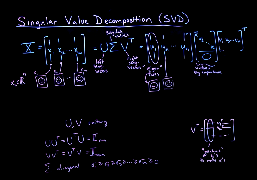
The Singular Value Decomposition of an $m\times n$ matrix $A$ is a factorization of the form:
$A=U\Sigma V^T$
where:

• $V$ is an $n\times n$ orthogonal matrix. Its columns, ${\mathbf{v}}_i$, are called the right singular vectors.
• $U$ is an $m\times m$ orthogonal matrix. Its columns, ${\mathbf{u}}_i$, are called the left singular vectors.
• $\Sigma$ is an $m\times n$ rectangular matrix that is zero everywhere except for its main diagonal. The diagonal entries, ${\sigma }_i$, are the singular values of $A$.

Now, let's derive how to find these three matrices. The following video walks through the entire derivation, which we will then formalize with rigorous definitions.

Formalizing the Construction

Let's consolidate the derivation from the video with formal mathematical statements.

1. Finding V and Σ:

   • Consider the $n\times n$ matrix $A^{T}A$. It is symmetric, so it has an orthonormal basis of eigenvectors and real eigenvalues.
   • Property: The eigenvalues of $A^{T}A$ are non-negative.
   • Proof: Let $(\lambda ,\mathbf{v})$ be an eigenpair of $A^{T}A$. Then $A^{T}A\mathbf{v}=\lambda \mathbf{v}$.
     $\Vert A\mathbf{v}{\Vert }^2=(A\mathbf{v}{)}^T(A\mathbf{v})={\mathbf{v}}^T{A}^{T}A\mathbf{v}={\mathbf{v}}^T(\lambda \mathbf{v})=\lambda {\mathbf{v}}^T\mathbf{v}=\lambda \Vert \mathbf{v}{\Vert }^2$
     Since norms are non-negative, $\lambda \Vert \mathbf{v}{\Vert }^2\ge 0$. As $\mathbf{v}$ is an eigenvector, $\Vert \mathbf{v}{\Vert }^2>0$, so we must have $\lambda \ge 0$.
   • We define the singular values of $A$, denoted ${\sigma }_i$, as the square roots of the eigenvalues of $A^{T}A$: ${\sigma }_i=\sqrt{{\lambda }_i}$. By convention, they are ordered such that ${\sigma }_1\ge {\sigma }_2\ge \cdots \ge 0$.
   • The right singular vectors, ${\mathbf{v}}_i$, are the corresponding orthonormal eigenvectors of $A^{T}A$. These form the columns of the matrix V.

2. Finding U:

   • Similarly, consider the $m\times m$ matrix $A{A}^T$. This is also a symmetric matrix with non-negative eigenvalues.
   • It can be shown that $A^{T}A$ and $A{A}^T$ have the same non-zero eigenvalues.
   • The left singular vectors, ${\mathbf{u}}_i$, are the orthonormal eigenvectors of $A{A}^T$. These form the columns of the matrix U.

The following resource provides a rigorous definition of the SVD and proves its existence.

Test your understanding!

Suppose $A=U\Sigma V^T$. You are told that the eigenvectors of $A^{T}A$ are the columns of $V$ and the eigenvalues are the squares of the singular values in $\Sigma$. Starting from $A=U\Sigma V^T$, can you prove this relationship by calculating $A^{T}A$?

Show answer

Starting with $A=U\Sigma V^T$, we compute its transpose:
$A^T=(U\Sigma V^T{)}^T=(V^T{)}^T{\Sigma }^T{U}^T=V{\Sigma }^T{U}^T$
Now, we can compute $A^{T}A$:
$A^{T}A=(V{\Sigma }^T{U}^T)(U\Sigma V^T)$
Since $U$ is an orthogonal matrix, $U^{T}U=I$. The expression simplifies to:
$A^{T}A=V({\Sigma }^T\Sigma )V^T$
Let's call the matrix $D={\Sigma }^T\Sigma$. Since $\Sigma$ is a rectangular diagonal matrix, $D$ will be a square diagonal matrix. Specifically, if $\Sigma$ is $m\times n$, then ${\Sigma }^T$ is $n\times m$, and $D$ is an $n\times n$ diagonal matrix whose entries are $d_{ii}={\sigma }_i^2$.

So we have $A^{T}A=VD{V}^T$. Since $V$ is orthogonal, $V^T=V^{-1}$, which means $A^{T}A=VD{V}^{-1}$. This is precisely the eigendecomposition of the matrix $A^{T}A$. The columns of $V$ are the eigenvectors, and the diagonal entries of $D$ (which are ${\sigma }_i^2$) are the corresponding eigenvalues. This confirms the relationship.

Properties and Geometric Intuition

A key part of the construction is that the vectors ${\mathbf{u}}_i$ defined as ${\mathbf{u}}_i=\frac{1}{{\sigma }_i}A{\mathbf{v}}_i$ (for ${\sigma }_i>0$) are guaranteed to be orthonormal. This remarkable property ensures that everything fits together perfectly. SVD can be geometrically interpreted as decomposing any linear transformation into a sequence of fundamental operations.

To prepare for our next lesson, it's useful to see one more way of writing the SVD.

Conclusion

In this lesson, we have formally defined the Singular Value Decomposition and rigorously derived its components. You now understand the deep connection between the SVD of a matrix $A$ and the eigendecomposition of the related symmetric matrices $A^{T}A$ and $A{A}^T$.

Key Takeaways:

• Any $m\times n$ matrix $A$ can be decomposed as $A=U\Sigma V^T$.
• V, the matrix of right singular vectors, is an $n\times n$ orthogonal matrix whose columns are the orthonormal eigenvectors of $A^{T}A$.
• U, the matrix of left singular vectors, is an $m\times m$ orthogonal matrix whose columns are the orthonormal eigenvectors of $A{A}^T$.
• Σ is an $m\times n$ rectangular diagonal matrix containing the non-negative singular values ${\sigma }_i$, which are the square roots of the eigenvalues of $A^{T}A$ (and $A{A}^T$).
• Geometrically, the SVD decomposes any linear transformation into a rotation, a scaling along the axes, and a second rotation.

Preview of the Next Lesson:
We ended by introducing the dyadic form of the SVD: $A={\sum }_{i=1}^r{\sigma }_i{\mathbf{u}}_i{\mathbf{v}}_i^T$. The singular values ${\sigma }_i$ are ordered by magnitude. This suggests that we can approximate the matrix $A$ by keeping only the first few terms in this sum—those corresponding to the largest singular values. In our next lesson, we will explore this idea and use SVD to perform low-rank approximation of a data matrix, a technique with profound applications from image compression to recommender systems.