Dimensionality Reduction with PCA

Hello! Welcome to your next lesson on eigenanalysis and its applications.

Introduction

In our previous lesson, we undertook a deep theoretical dive to derive the formulation of Principal Component Analysis (PCA). We rigorously proved, from two different perspectives, that the principal components of a dataset are precisely the eigenvectors of its covariance matrix, and the corresponding eigenvalues represent the variance captured by each component.

Today, we transition from theory to practice. Our learning outcome is to apply PCA to a data matrix to perform dimensionality reduction. We will build on the "why" you learned last time to establish the "how"—a concrete, step-by-step algorithm for using PCA. You will learn how to process a dataset, extract the principal components, decide how many components to keep, and transform the data into a lower-dimensional representation.

Let's begin by visually recalling the core idea.

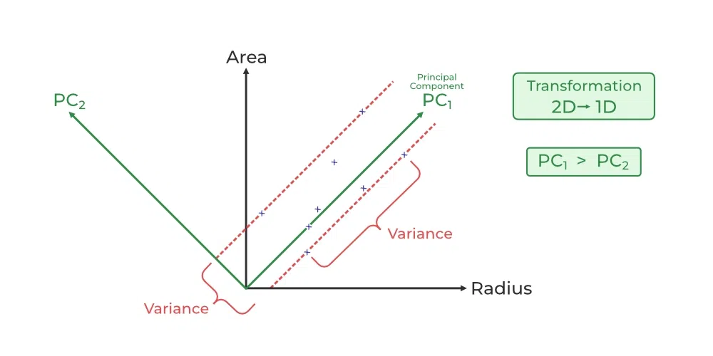
The PCA Algorithm: From Data to Components

Applying PCA involves a sequence of clear, well-defined steps. We'll use the standard machine learning data convention where our data matrix $X$ has dimensions $n\times m$, with $n$ being the number of samples (data points) and $m$ being the number of features.

Step 1: Center the Data

The first, and crucial, step is to center the data by subtracting the mean of each feature. For each feature $j$ (i.e., each column of $X$), we compute its mean ${\mu }_j$ and subtract it from every entry in that column.

$X_{\text{centered}}[i,j]=X[i,j]-{\mu }_j$

This ensures that each feature has a mean of zero. This is a necessary prerequisite because the covariance matrix, which measures how features vary together, is defined in terms of deviations from the mean.

Step 2: Compute the Covariance Matrix

With the centered data matrix $X_{\text{centered}}$, we can now compute the $m\times m$ sample covariance matrix, which we'll denote as $S$.

$S=\frac{1}{n-1}{X}_{\text{centered}}^T{X}_{\text{centered}}$

Let's break this down:

• $X_{\text{centered}}^T$ has dimensions $m\times n$.
• $X_{\text{centered}}$ has dimensions $n\times m$.
• The product $X_{\text{centered}}^T{X}_{\text{centered}}$ results in an $m\times m$ matrix.
• The $ij$-th entry of this matrix is the dot product of the $i$-th and $j$-th columns (features) of $X_{\text{centered}}$, which, when scaled by $\frac{1}{n-1}$, gives the covariance between feature $i$ and feature $j$. The diagonal entries are the variances.

Step 3: Eigendecomposition of the Covariance Matrix

This is where the theory from our last lesson comes into play. We perform an eigendecomposition of the symmetric covariance matrix $S$.

$S=U\Lambda U^T$

• $\Lambda$ is a diagonal matrix containing the eigenvalues (${\lambda }_1,{\lambda }_2,\dots ,{\lambda }_m$) of $S$.
• $U$ is an orthonormal matrix whose columns (${\mathbf{u}}_1,{\mathbf{u}}_2,\dots ,{\mathbf{u}}_m$) are the corresponding eigenvectors of $S$.

As we proved, these eigenvectors ${\mathbf{u}}_i$ are the principal components of our data, and the eigenvalues ${\lambda }_i$ are the variances captured by each component.

Step 4: Sort Components and Project the Data

The eigenvalues tell us the importance of each principal component. To perform dimensionality reduction, we first sort the eigenvalues in descending order and sort the eigenvectors (principal components) accordingly.

Let's say we decide to reduce the dimensionality from $m$ to $k$ (where $k<m$). We select the first $k$ principal components corresponding to the $k$ largest eigenvalues. Let's form a matrix $U_k$ of size $m\times k$ whose columns are these top $k$ principal components.

To get our new, lower-dimensional data representation $Z$, we project the centered data onto these components:

$Z=X_{\text{centered}}{U}_k$

• $X_{\text{centered}}$ is $n\times m$.
• $U_k$ is $m\times k$.
• The resulting matrix $Z$ is $n\times k$. Each row of $Z$ is the new $k$-dimensional representation of the corresponding original data point.

Performing Dimensionality Reduction

The most critical decision in applying PCA is choosing $k$, the number of components to keep. How do we make this choice in a principled way?

We use the concept of explained variance. The total variance in the data is the sum of all the eigenvalues: ${\sum }_{i=1}^m{\lambda }_i$. The proportion of total variance explained by the $i$-th principal component is:

${\text{Explained Variance}}_i=\frac{{\lambda }_i}{{\sum }_{j=1}^m{\lambda }_j}$

To choose $k$, we typically look at the cumulative explained variance. We calculate the sum of the explained variance for the top $k$ components and keep enough components to exceed a certain threshold, often 95% or 99%.

For a deeper dive into the algorithm and the practicalities of dimensionality reduction, the following resources are excellent.

Test your understanding!

You have a dataset with 5 features ($m=5$). After running PCA, you get the following eigenvalues: ${\lambda }_1=50$, ${\lambda }_2=25$, ${\lambda }_3=15$, ${\lambda }_4=8$, ${\lambda }_5=2$.

1. What is the total variance in the data?
2. What percentage of the total variance is explained by the first principal component (PC1)?
3. If you want to retain at least 90% of the total variance, how many principal components ($k$) should you keep?

Show answer

1. The total variance is the sum of the eigenvalues: $50+25+15+8+2=100$.
2. PC1 explains $\frac{50}{100}=50\%$ of the total variance.
3. Let's compute the cumulative variance:
   • PC1: 50%
   • PC1 + PC2: $50+25=75\%$
   • PC1 + PC2 + PC3: $75+15=90\%$
   • PC1 + PC2 + PC3 + PC4: $90+8=98\%$
     You should keep 3 principal components to retain exactly 90% of the variance, or 4 to be strictly above 90%. In practice, you would typically choose $k=4$ to ensure the threshold is met and exceeded.

A Complete Example: PCA in Action

Let's see this entire process applied to a dataset. The following video provides an excellent walkthrough, demonstrating how PCA can find the underlying structure in noisy, high-dimensional data.

An Alternative Method: The SVD Connection

While computing the eigendecomposition of the covariance matrix is the definitional way to perform PCA, it is not always the most numerically stable or efficient method in practice. A more robust approach uses the Singular Value Decomposition (SVD), which we will study in detail in our next lesson.

For now, it is sufficient to know that you can perform PCA directly by taking the SVD of the centered data matrix $X_{\text{centered}}$.

The key takeaway is that if $X_{\text{centered}}=U\Sigma V^T$ (the SVD of the centered data), then:

• The columns of $V$ are the principal components (the same eigenvectors of $S$).
• The singular values in the diagonal matrix $\Sigma$ are related to the eigenvalues of $S$ by ${\lambda }_i=\frac{{\sigma }_i^2}{n-1}$. This means the squared singular values also tell you how variance is distributed across the components.

This deep connection between eigenanalysis, PCA, and SVD is a cornerstone of linear algebra in data science. For your interest, the Shlens tutorial (LINK, Section VI) provides a full mathematical derivation of this relationship.

Conclusion

In this lesson, we have translated the theory of PCA into a practical algorithm for dimensionality reduction. You now have the complete picture, from the foundational mathematics to the applied methodology.

Key Takeaways:

• The PCA algorithm consists of four main steps: centering the data, computing the covariance matrix, performing eigendecomposition on this matrix, and projecting the data onto the top-ranked eigenvectors (principal components).
• The number of components to retain, $k$, is chosen based on the desired cumulative explained variance, which is calculated from the eigenvalues.
• Applying PCA transforms the data into a new, lower-dimensional space where the new features (the principal components) are uncorrelated and ordered by the amount of variance they capture.
• While PCA is defined by the eigendecomposition of the covariance matrix, it can be more robustly computed using the Singular Value Decomposition (SVD) of the data matrix.

Preview of the Next Lesson:
We've just seen a glimpse of how SVD relates to PCA. In our next lesson, we will formally define the Singular Value Decomposition (SVD). You will learn about its constituent matrices ($U$, $\Sigma$, and $V$) and their fundamental properties. We will explore why SVD is arguably one of the most important matrix decompositions in all of data analysis and machine learning.