PCA: Eigendecomposition of the Covariance Matrix

Hello! Welcome to the fifth lesson in our module on eigenanalysis.

Introduction

In our last lesson, we established the theory of matrix diagonalization. We proved that an $n\times n$ matrix $A$ is diagonalizable if and only if it has $n$ linearly independent eigenvectors, and we saw that this allows for the powerful eigendecomposition $A=PD{P}^{-1}$. We noted that symmetric matrices are a special case, as they are always diagonalizable and have an orthonormal basis of eigenvectors.

Today, we will apply this powerful decomposition to derive one of the most fundamental techniques in data science: Principal Component Analysis (PCA). The learning outcome for this lesson is to use the eigendecomposition of a covariance matrix to derive the formulation of Principal Component Analysis (PCA).

We will start by framing the intuitive goal of PCA—finding the directions of maximum variance in a dataset. We will then formalize this goal mathematically and, through two distinct but complementary derivations, prove that the solution to this problem is found by computing the eigenvectors of the data's covariance matrix. This lesson will provide the complete theoretical "why" behind PCA.

1. The Goal of PCA and the Covariance Matrix

Imagine you have a dataset with many features (i.e., it's high-dimensional). Many of these features might be correlated, meaning they contain redundant information. The goal of PCA is to find a new, smaller set of uncorrelated features, called principal components, that capture the maximum possible variance from the original data. In essence, it's a method for dimensionality reduction that aims to lose the least amount of information.

The central mathematical object in PCA is the covariance matrix.

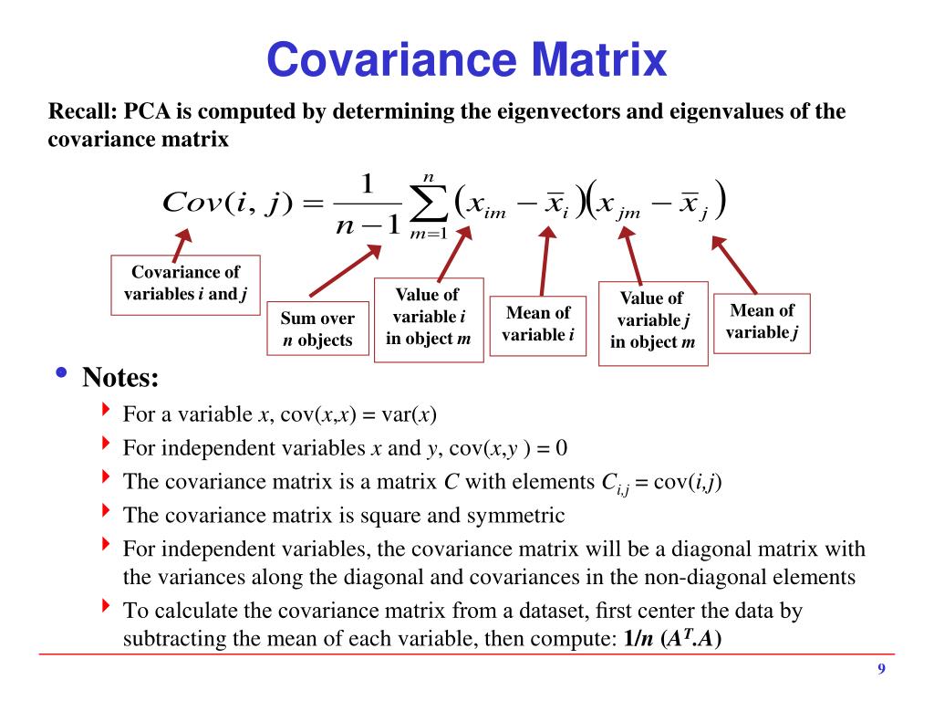
Let's consider a dataset represented by a matrix $X$ of size $m\times n$, where $m$ is the number of features and $n$ is the number of data points. After centering the data (subtracting the mean from each feature), the covariance matrix $S$ is a square $m\times m$ matrix calculated as:
$S=\frac{1}{n-1}X{X}^T$
The key properties of the covariance matrix $S$ are:

• Symmetry: $S=S^T$. The covariance between feature $i$ and feature $j$ is the same as between $j$ and $i$.
• Diagonal entries: The diagonal elements $S_{ii}$ are the variances of each feature.
• Off-diagonal entries: The off-diagonal elements $S_{ij}$ are the covariances between features $i$ and $j$.

From our last lesson, we know that symmetric matrices are special. A symmetric matrix is always diagonalizable, and its eigenvectors form an orthonormal basis. This property is the linchpin of the PCA derivation.

2. Derivation 1: PCA as Variance Maximization

The most common way to derive PCA is to frame it as a constrained optimization problem. We want to find the direction in our feature space (represented by a unit vector $\mathbf{u}$) along which the projected data has the greatest possible variance.

Let's formalize this.

1. Projection: A data point $\mathbf{x}$ (a column vector) is projected onto the direction $\mathbf{u}$. The coordinate of the projection is given by the dot product ${\mathbf{x}}^T\mathbf{u}$.
2. Variance of Projections: We want to find the variance of these projected coordinates over the whole dataset.
3. Objective: Maximize this variance.
4. Constraint: The direction $\mathbf{u}$ must be a unit vector, i.e., ${\mathbf{u}}^T\mathbf{u}=1$. Without this constraint, we could make the variance arbitrarily large just by scaling $\mathbf{u}$.

The following video walks through this derivation step-by-step.

Let's summarize the key steps of the derivation you just saw.

1. Expressing the Variance: The variance of the data projected onto a direction $\mathbf{u}$ is neatly expressed as:
   $\text{Var}(\text{projection})={\mathbf{u}}^{T}S\mathbf{u}$
   where $S$ is the covariance matrix.

2. Constrained Optimization: The problem becomes:
   ${\max }_{\mathbf{u}}{\mathbf{u}}^{T}S\mathbf{u}\text{subject to}{\mathbf{u}}^T\mathbf{u}=1$

3. Lagrangian Formulation: We introduce a Lagrange multiplier $\lambda$ and form the Lagrangian:
   $\mathcal{L}(\mathbf{u},\lambda )={\mathbf{u}}^{T}S\mathbf{u}-\lambda ({\mathbf{u}}^T\mathbf{u}-1)$

4. Solving for the Optimum: To find the maximum, we take the gradient with respect to $\mathbf{u}$ and set it to zero:
   ${\nabla }_{\mathbf{u}}\mathcal{L}=2S\mathbf{u}-2\lambda \mathbf{u}=0$
   This simplifies to:
   $S\mathbf{u}=\lambda \mathbf{u}$

This is precisely the eigenvalue equation for the covariance matrix $S$. This proves that the directions of maximum variance must be the eigenvectors of the covariance matrix.

But which eigenvector? Let's substitute this result back into our expression for the variance:
$\text{Variance}={\mathbf{u}}^{T}S\mathbf{u}={\mathbf{u}}^T(\lambda \mathbf{u})=\lambda ({\mathbf{u}}^T\mathbf{u})=\lambda (1)=\lambda$
The variance captured by an eigenvector $\mathbf{u}$ is its corresponding eigenvalue $\lambda$. Therefore, to maximize the variance, we must choose the eigenvector with the largest eigenvalue. This eigenvector is the first principal component (PC1). The second principal component is the eigenvector with the second-largest eigenvalue, and so on.

3. Derivation 2: PCA as Diagonalization

There is another, equally powerful way to derive PCA that connects directly to our work on diagonalization from the previous lesson. This approach frames the goal not as maximizing variance, but as finding a new basis where the features are uncorrelated.

If the new features are uncorrelated, their covariance matrix must be a diagonal matrix (all off-diagonal covariance terms are zero).

Let's walk through the logic from that reading.

1. Define the Transformation: Let the original data be $X$ with covariance matrix $S=\frac{1}{n-1}X{X}^T$. Let $P$ be an orthonormal transformation matrix where each row is a new basis vector. The transformed data is $Y=PX$.

2. Covariance of Transformed Data: The covariance matrix of the new data, $C_Y$, is:
   $C_Y=\frac{1}{n-1}Y{Y}^T=\frac{1}{n-1}(PX)(PX{)}^T=\frac{1}{n-1}PX{X}^T{P}^T=P\left(\frac{1}{n-1}X{X}^T\right)P^T=PS{P}^T$

3. The Goal: We want $C_Y$ to be a diagonal matrix, which we'll call $D$. So our goal is to find an orthonormal matrix $P$ such that:
   $D=PS{P}^T$

4. Connecting to Eigendecomposition: Since $P$ is orthonormal, $P^{-1}=P^T$. We can right-multiply by $P$ (which is $P^{T^T}$) to get:
   $DP=PS{P}^{T}P⟹DP=PS$
   And by pre-multiplying by $P^T$, we get:
   $P^{T}DP=P^{T}PS⟹S=P^{T}DP$

This final equation, $S=P^{T}DP$, is exactly the eigendecomposition of the symmetric matrix $S$ that we studied in the last lesson (where the columns of $P^T$ are the eigenvectors of $S$, and $D$ is the diagonal matrix of eigenvalues).

Therefore, the rows of the transformation matrix $P$—our principal components—must be the orthonormal eigenvectors of the covariance matrix $S$. This second derivation beautifully confirms our first result: finding a basis that uncorrelates the data is equivalent to finding the eigenvectors of the covariance matrix.

4. Synthesis and Properties

Both derivations lead to the same fundamental conclusion:

The principal components of a dataset are the orthonormal eigenvectors of its covariance matrix. The first principal component is the eigenvector corresponding to the largest eigenvalue, the second principal component corresponds to the second-largest eigenvalue, and so on.

This is the core theoretical formulation of PCA.

A few important properties emerge from this derivation:

• Variance Explained: The eigenvalue ${\lambda }_i$ corresponding to the $i$-th principal component ${\mathbf{u}}_i$ represents the variance of the data projected onto that component.
• Total Variance: The sum of all the eigenvalues is equal to the trace (sum of the diagonal elements) of the original covariance matrix $S$. This means the sum of the eigenvalues is the total variance in the original data.
  $\text{Total Variance}={\sum }_{i=1}^m\text{Var}(X_i)=\text{tr}(S)={\sum }_{i=1}^m{\lambda }_i$
• Uncorrelated Components: As shown in the second derivation, the new features (projections onto the principal components) are mutually uncorrelated. Their covariance matrix is diagonal.

Conclusion

In this lesson, we have rigorously derived the mathematical formulation of Principal Component Analysis. By connecting the intuitive goal of finding directions of maximum data variance to the formal machinery of linear algebra, we have proven a cornerstone result of machine learning.

Key Takeaways:

• PCA seeks to find a set of orthogonal axes (principal components) that capture the maximum variance in a dataset.
• We proved through two different derivations (variance maximization and covariance diagonalization) that these principal components are the eigenvectors of the data's covariance matrix.
• The eigenvalues of the covariance matrix quantify the variance captured by each corresponding principal component, allowing us to rank them by importance.
• The eigendecomposition of the covariance matrix, $S=UD{U}^T$, provides the complete solution: $U$ contains the principal components, and $D$ contains their associated variances.

Preview of the Next Lesson:
Now that we have established the "why" and "what" of PCA, the next lesson will focus on the "how." We will move from derivation to application, learning how to take a data matrix, compute its principal components, and use them to perform dimensionality reduction. We will discuss the practical steps of choosing how many components to retain and visualizing the transformed data.