Low-Rank Approximation with SVD

Hello! Let's dive into the final lesson of our module on Eigenanalysis and Matrix Decompositions.

Introduction

In our previous lesson, we formally defined the Singular Value Decomposition (SVD), $A=U\Sigma V^T$, and saw that any matrix $A$ can be expressed as a sum of rank-one matrices, known as its dyadic form:
$A={\sum }_{i=1}^r{\sigma }_i{\mathbf{u}}_i{\mathbf{v}}_i^T$
where $r$ is the rank of $A$, and the singular values ${\sigma }_i$ are ordered from largest to smallest. This structure is not just a mathematical curiosity; it's the key to one of the most powerful applications of SVD.

Today's learning outcome is to use SVD to perform low-rank approximation of a data matrix. We will see that by simply truncating this sum—keeping only the terms with the largest singular values—we can create a lower-rank matrix that is the best possible approximation of the original. This concept is fundamental to applications like image compression, recommender systems, and noise reduction in data.

The Construction of a Low-Rank Approximation

The dyadic form of the SVD gives us a way to build the matrix $A$ piece by piece. The first term, ${\sigma }_1{\mathbf{u}}_1{\mathbf{v}}_1^T$, represents the most significant rank-one component of the matrix. Each subsequent term adds a layer of finer detail. This suggests that if we want to capture the "essence" of the matrix while discarding less important information (or noise), we can just keep the first $k$ terms of the sum, where $k<r$.

We define the best rank-k approximation of $A$, denoted $A_k$, as:
$A_k={\sum }_{i=1}^k{\sigma }_i{\mathbf{u}}_i{\mathbf{v}}_i^T$
This new matrix $A_k$ has, by construction, a rank of $k$.

Another way to think about this is in terms of the full $A=U\Sigma V^T$ factorization. To get $A_k$, we take the matrix $\Sigma$ and set all singular values after the k-th one to zero. Let's call this new matrix ${\Sigma }_k$. Then:
$A_k=U{\Sigma }_k{V}^T$

The following image provides a clear visual summary of this process.

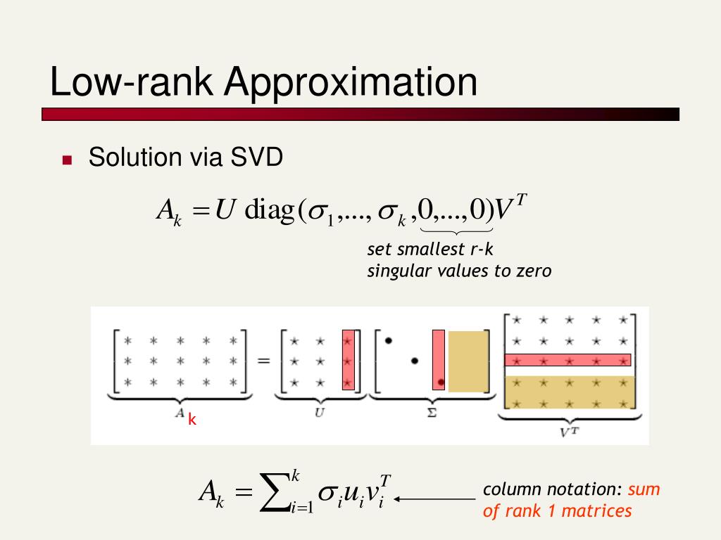
But what do we mean by the "best" approximation? To answer this, we need a way to measure the size of the error, which is the difference matrix $A-A_k$. This brings us to the concept of matrix norms.

Measuring Error with Matrix Norms

Just as a vector norm measures the length of a vector, a matrix norm measures the "size" or "magnitude" of a matrix. The idea of the "best" approximation is formalized as finding a rank-$k$ matrix $B$ that minimizes the norm of the error, $\Vert A-B\Vert$.

While there are many matrix norms, the Eckart-Young theorem holds for two particularly important ones that are defined using singular values.

From the reading, the two key norms are:

1. The Spectral Norm (2-norm): $\Vert A{\Vert }_2={\sigma }_1(A)$, the largest singular value of $A$. It measures the maximum "stretching" effect the matrix has on any unit vector.
2. The Frobenius Norm: $\Vert A{\Vert }_F=\sqrt{{\sum }_{i=1}^m{\sum }_{j=1}^n|a_{ij}{|}^2}=\sqrt{\text{Tr}(A^{T}A)}$. This is like treating the matrix as one long vector and calculating its standard Euclidean length. A key property is that $\Vert A{\Vert }_F^2={\sum }_{i=1}^r{\sigma }_i^2$.

With these tools, we can now state the central theorem of this lesson.

The Eckart-Young-Mirsky Theorem: The Optimality of SVD

The main result that makes SVD so useful for approximation is the Eckart-Young-Mirsky Theorem. It states that the matrix $A_k$ we constructed by truncating the SVD is not just a good approximation of $A$, but it is the best possible rank-$k$ approximation.

Now, for the formal statement and proof. The theorem provides an exact formula for the minimum possible error.

Theorem (Eckart-Young-Mirsky):
Let $A$ be an $m\times n$ matrix of rank $r$, and let $A_k={\sum }_{i=1}^k{\sigma }_i{\mathbf{u}}_i{\mathbf{v}}_i^T$ be its rank-$k$ approximation from SVD, with $k\le r$. Then for any matrix $B$ of rank at most $k$:

1. Spectral Norm: $\Vert A-B{\Vert }_2\ge \Vert A-A_k{\Vert }_2={\sigma }_{k+1}$
2. Frobenius Norm: $\Vert A-B{\Vert }_F\ge \Vert A-A_k{\Vert }_F=\sqrt{{\sum }_{i=k+1}^r{\sigma }_i^2}$

This theorem is profound: it tells us that no other rank-$k$ matrix can get closer to $A$ than the one we build from its SVD. The error of our approximation is precisely determined by the singular values we chose to discard.

Since you've requested mathematical rigor, we will now examine the proof of this theorem.

How to Choose the Rank k?

The theorem provides the optimal approximation for a given rank $k$, but it doesn't tell us how to choose $k$. This choice involves a trade-off:

• A small $k$ gives high compression/dimensionality reduction but a less accurate approximation.
• A large $k$ gives a very accurate approximation but less compression.

In practice, a common heuristic is to choose $k$ such that a certain percentage (e.g., 90%) of the "energy" of the matrix is retained. The total energy is defined as the squared Frobenius norm, $\Vert A{\Vert }_F^2={\sum }_{i=1}^r{\sigma }_i^2$.

The fraction of energy retained by a rank-$k$ approximation is:
$\frac{{\sum }_{i=1}^k{\sigma }_i^2}{{\sum }_{i=1}^r{\sigma }_i^2}$
One can then plot this cumulative energy against $k$ and choose a $k$ at the "elbow" of the curve, where adding more components yields diminishing returns.

This idea of retaining variance should be familiar from our discussion on PCA. Indeed, for a centered data matrix, the squared singular values from SVD are directly proportional to the eigenvalues of the covariance matrix used in PCA. SVD provides a more direct and numerically stable way to achieve the same goal.

Conclusion

This lesson completes our deep dive into SVD and its role in creating optimal low-rank approximations. This is a cornerstone of modern data analysis, enabling efficient handling and interpretation of large-scale data.

Key Takeaways:

• The SVD of a matrix $A$ can be used to construct a rank-$k$ approximation $A_k$ by summing the first $k$ terms of its dyadic expansion.
• The Eckart-Young-Mirsky Theorem guarantees that $A_k$ is the best possible rank-$k$ approximation to $A$, minimizing the error in both the spectral and Frobenius norms.
• The approximation error is determined entirely by the singular values that are discarded: $\Vert A-A_k{\Vert }_2={\sigma }_{k+1}$ and $\Vert A-A_k{\Vert }_F=\sqrt{{\sum }_{i=k+1}^r{\sigma }_i^2}$.
• The choice of rank $k$ is a practical decision based on the desired balance between accuracy and compression, often guided by the concept of "retained energy."

Preview of the Next Module:
We have now concluded our module on Eigenanalysis and Matrix Decompositions. You have built a solid foundation in the linear algebra that underpins many machine learning algorithms.

Our next module, Multivariate Calculus for Machine Learning, will equip us with a new set of essential tools. We will move from the world of linear transformations to the world of functions and optimization. You will learn to compute partial derivatives, gradients, and Hessian matrices. These concepts are the language of optimization, allowing us to find the minimum of a function—for instance, to find the model parameters that minimize a cost function. This is the mathematical engine that drives the training of almost every machine learning model.