Defining a Multilayer Perceptron with `torch.nn.Module`

Welcome back. In the previous lesson, you used autograd to obtain gradients for weights and biases that you created yourself. Now you will put those computations inside a reusable PyTorch model. By the end of this lesson, you will be able to define a multilayer perceptron (MLP) as a subclass of torch.nn.Module, pass a batch through it, and inspect the parameters it owns.

An MLP will be useful throughout this course: first as a model for supervised learning, and later as a component of agents that estimate values or choose actions. For now, the goal is to define its structure correctly—not to train it yet.

From tensor operations to a model

An MLP takes a vector of input features, combines them with learned weights and biases, applies a nonlinear activation, and produces an output vector. The diagram below shows one hidden layer. Each connection between layers corresponds to part of a learned weight matrix.

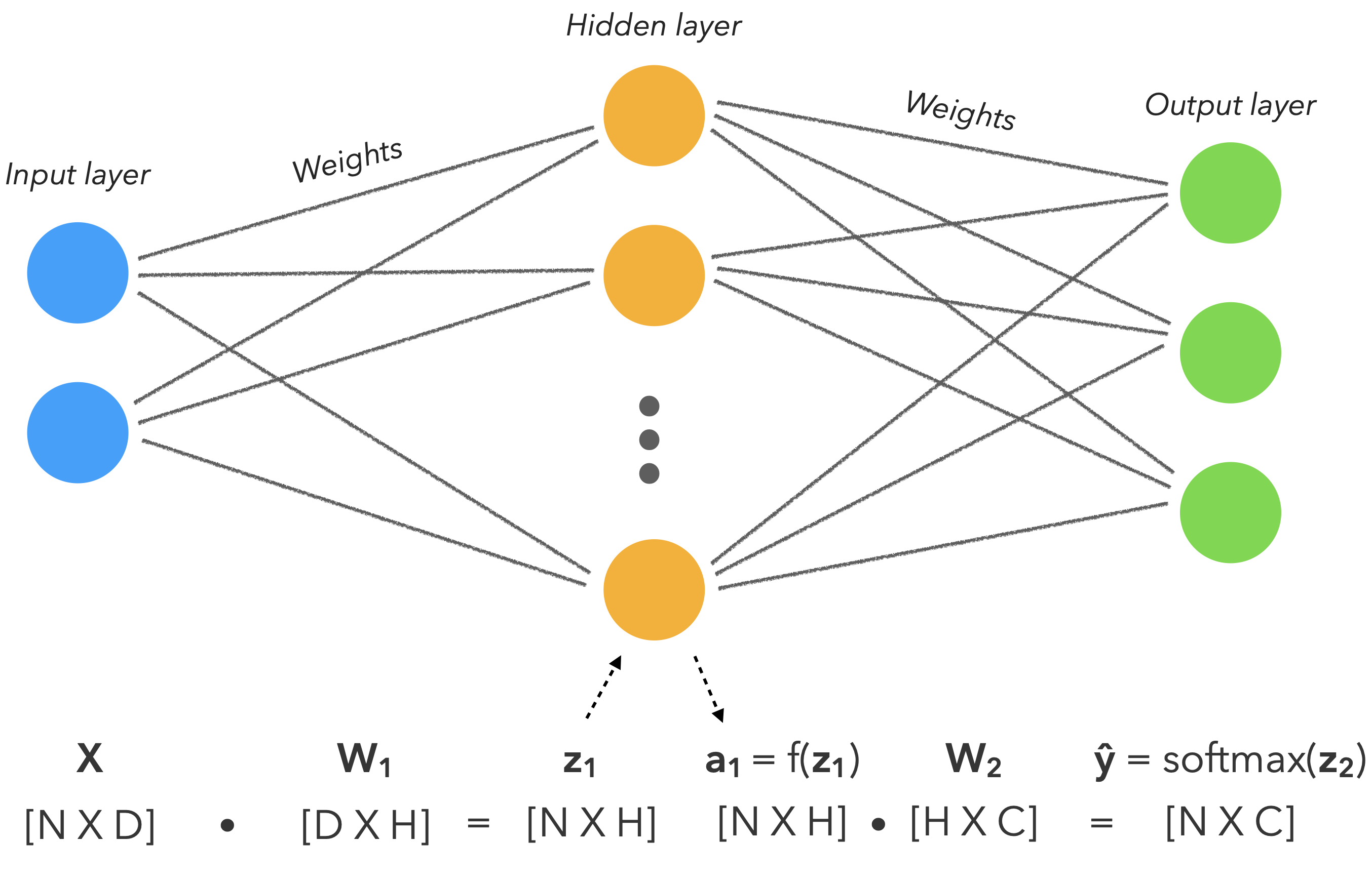
If a batch contains $N$ examples, each with $D$ features, the input has shape $(N,D)$. A hidden layer with $H$ units produces $(N,H)$; an output layer with $C$ units produces $(N,C)$. The activation between the layers matters: without a nonlinearity, consecutive linear layers with biases could be combined into a single affine transformation.

Watch the model-building portion of Aladdin Persson’s Pytorch Neural Network example. It demonstrates the two parts you will write: an initializer that creates layers and a forward method that uses them.

In PyTorch, nn.Linear(D, H) creates a layer that accepts $D$ features and returns $H$ features. It stores its own weight and bias. With the usual batch shape $(N,D)$, the calculation is:

One shape detail can be surprising: although the diagram writes a matrix of shape $(D,H)$ to the right of $X$, PyTorch stores nn.Linear(D, H).weight with shape $(H,D)$ and uses its transpose in this calculation.

Define the class

Read the indicated parts of PyTorch’s official Build the Neural Network tutorial. Its example starts with $28\times 28$ images, so it includes a flattening layer. Our first model will accept feature vectors that are already flat.

Let us build an MLP with four input features, eight hidden units, and three outputs. Those numbers make the shapes easy to inspect; the same class can also be instantiated with other widths.

import torch
from torch import nn


class MLP(nn.Module):
    def __init__(self, input_dim: int, hidden_dim: int, output_dim: int):
        super().__init__()
        self.fc1 = nn.Linear(input_dim, hidden_dim)
        self.activation = nn.ReLU()
        self.fc2 = nn.Linear(hidden_dim, output_dim)

    def forward(self, x: torch.Tensor) -> torch.Tensor:
        x = self.fc1(x)
        x = self.activation(x)
        x = self.fc2(x)
        return x


model = MLP(input_dim=4, hidden_dim=8, output_dim=3)
print(model)

class MLP(nn.Module) makes MLP a subclass of PyTorch’s model base class. Calling super().__init__() initializes the base class before you assign layers to self. The assignments create persistent submodules: fc1 and fc2 hold trainable weights and biases, while activation applies ReLU without trainable parameters.

The forward method defines what happens each time the model receives an input. Here, fc1 produces eight values per example, ReLU replaces negative values with zero, and fc2 produces three output values. The same layers—and therefore the same stored parameters—are reused on every call. We do not create new nn.Linear layers inside forward.

You could put these three operations in an nn.Sequential container, as the official tutorial does. Writing them out in forward makes the subclass’s responsibilities especially visible: __init__ defines the components; forward specifies the computation.

Call the model and check its shapes

Use the model instance like a function. PyTorch then invokes forward through the module’s normal calling machinery; do not call model.forward(x) directly.

x = torch.randn(5, 4)   # 5 examples, 4 features each
scores = model(x)

print(x.shape)          # torch.Size([5, 4])
print(scores.shape)     # torch.Size([5, 3])

The batch dimension remains $5$. The first linear layer changes the feature dimension from $4$ to $8$, ReLU leaves the shape unchanged, and the second linear layer changes it from $8$ to $3$. If x instead had shape (5, 6), the first layer would reject it: its in_features is $4$.

The returned values are raw outputs, often called scores or logits when used for classification. The diagram shows a softmax after its output layer, but this class deliberately stops at the final linear layer. Whether to transform those outputs depends on the task and loss function; you will make that choice later in the course.

If your starting data were images of shape (batch, height, width), you would need to flatten each image into a feature vector first, as in the official tutorial. For an input already shaped (batch, features), adding nn.Flatten would be unnecessary.

Inspect what the model owns

In the previous lesson, you marked individual tensors with requires_grad=True. Here, each nn.Linear creates its trainable parameters for you. Because those layers were assigned as attributes of an nn.Module, PyTorch registers their parameters and makes them available through model.parameters() and model.named_parameters().

for name, parameter in model.named_parameters():
    print(name, tuple(parameter.shape), parameter.requires_grad)

For this model, the reported names and shapes are:

fc1.weight (8, 4) True
fc1.bias   (8,)   True
fc2.weight (3, 8) True
fc2.bias   (3,)   True

ReLU does not appear because it has no weights or biases. The model has $8\times 4+8=40$ parameters in fc1 and $3\times 8+3=27$ in fc2, for 67 trainable numbers in all. Checking these shapes is a useful way to catch a reversed layer dimension or a missing layer before training.

Subclassing nn.Module provides the model structure and parameter registration; autograd still computes gradients through the tensor operations, just as it did last lesson. Defining and calling a model does not itself compute a loss, run a backward pass, or update its weights.

Conclusion

To define an MLP in PyTorch, subclass nn.Module, call super().__init__(), create layers as attributes in __init__, and compose them in forward. Call the instance with model(x), check that its batch and feature dimensions match your intent, and use named_parameters() to verify the registered weights and biases.

You now have a model that produces outputs and exposes trainable parameters. Next, you will compute a loss from those outputs and use a PyTorch optimizer to update the parameters.