Computing Loss and Updating Parameters with PyTorch Optimizers

Welcome back. Last lesson, you defined an MLP that turns a batch of inputs into raw output scores, and you checked that PyTorch registered its weights and biases. Earlier, you used autograd to compute gradients. Today, you will connect those pieces: compare the model’s outputs with targets, compute a loss, and use an optimizer to change the model’s parameters.

We will use the same four-input, eight-hidden-unit, three-output MLP for a small classification task. By the end, you will have a working training loop, not just a model that makes predictions.

Turn model outputs into a loss

A forward pass gives us scores, but it does not tell us how well the model did. A loss function compares those scores with the correct targets and returns a number we want to reduce.

Watch the selected parts of Patrick Loeber’s PyTorch Tutorial 06 - Training Pipeline: Model, Loss, and Optimizer. The example is simpler than our MLP, which makes the division of work among the model, loss function, and optimizer easier to see.

For our three-output model, we will treat the outputs as classification logits: three unrestricted scores per example, one for each class. We will use nn.CrossEntropyLoss() to compare them with class labels. With a batch of $N$ examples:

• The model output has shape $(N,3)$ and a floating-point dtype.
• The target has shape $(N,)$, contains integer class indices 0, 1, or 2, and has dtype torch.long.
• The loss is a scalar tensor. With the default settings, it averages the examples’ losses.

Pass the raw logits to CrossEntropyLoss; do not apply softmax in the model first. The loss function handles the conversion it needs internally. For a regression task, a common alternative is nn.MSELoss(), which compares numerical predictions with numerical targets. We will examine task-specific choices more carefully later; for now, what matters is that the loss connects your model’s output to a trainable objective.

Give gradients to an optimizer

Read the focused portions of PyTorch’s official Optimizing Model Parameters tutorial. They describe both the purpose of the loss and the three operations that turn it into a parameter update.

For basic stochastic gradient descent (SGD), the idea behind optimizer.step() is to move each registered parameter $p$ opposite its loss gradient:

where $\eta$ is the learning rate. You choose the learning rate when you create the optimizer; PyTorch then applies the updates to the parameters you passed it.

The training-loop image shows where each operation belongs:

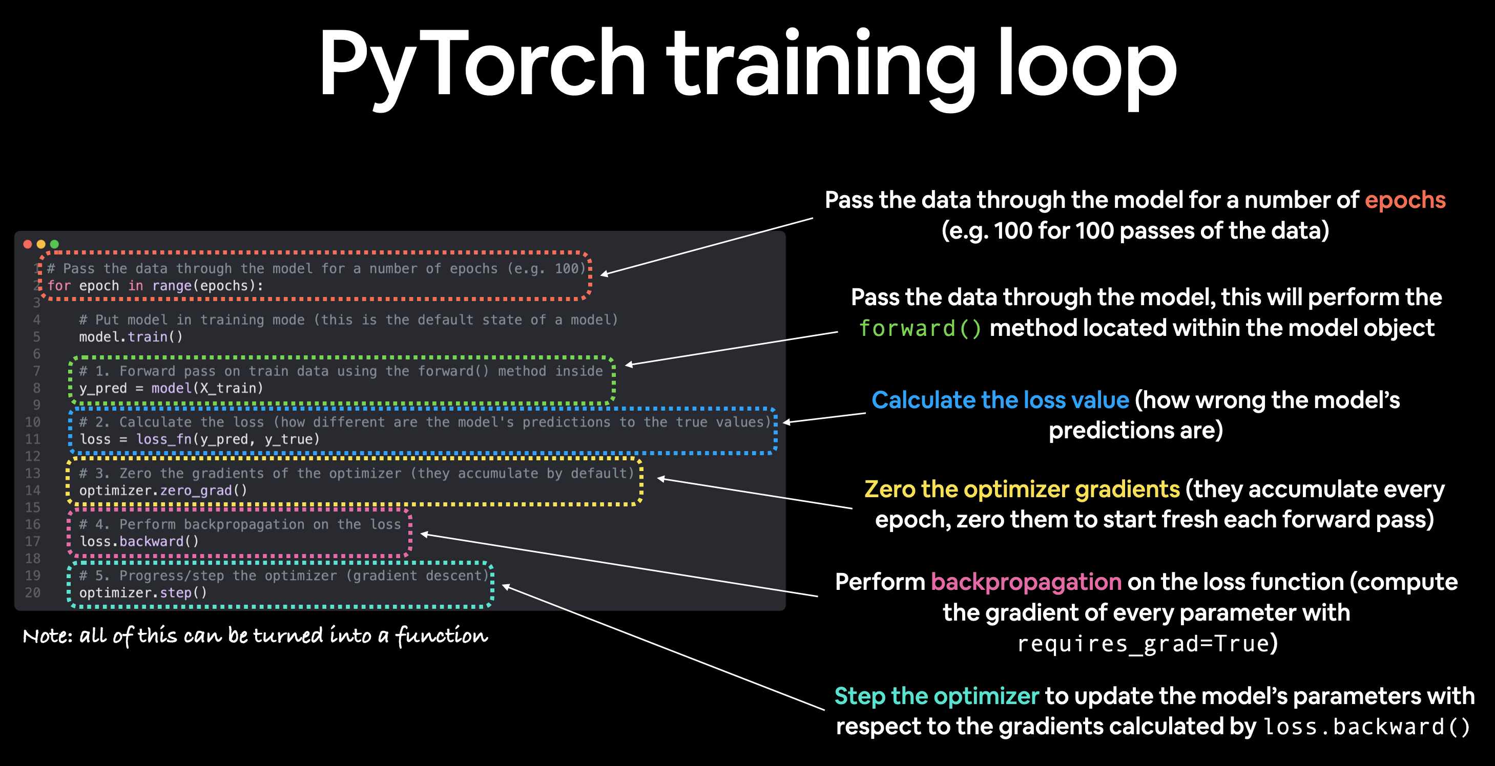
The crucial distinction is that loss.backward() computes gradients and places them in parameters’ .grad attributes. optimizer.step() uses those gradients to update parameters; it does not compute them. PyTorch accumulates gradients by default, so optimizer.zero_grad() clears old gradients before the next backward pass. In the image, there is one update per epoch. If an epoch contains many batches, clear gradients for each update, not only once per epoch.

You may see zero_grad() immediately after step() in some tutorials. That can also prepare for the next pass. We will put it before the forward pass so that each update visibly starts with cleared gradients.

Make one update with the MLP

The following code is self-contained, though the class is the same one you built last lesson. Our six examples all fit in one batch. Their labels indicate which of three classes each example belongs to; the fourth input feature simply gives the small dataset a little variation.

import torch
from torch import nn


class MLP(nn.Module):
    def __init__(self, input_dim: int, hidden_dim: int, output_dim: int):
        super().__init__()
        self.fc1 = nn.Linear(input_dim, hidden_dim)
        self.activation = nn.ReLU()
        self.fc2 = nn.Linear(hidden_dim, output_dim)

    def forward(self, x: torch.Tensor) -> torch.Tensor:
        return self.fc2(self.activation(self.fc1(x)))


X = torch.tensor([
    [2.0, 0.0, 0.0, 0.0],
    [1.0, 0.5, 0.0, 0.0],
    [0.0, 2.0, 0.0, 0.0],
    [0.0, 1.0, 0.5, 0.0],
    [0.0, 0.0, 2.0, 0.0],
    [0.0, 0.0, 1.0, 0.5],
])
y = torch.tensor([0, 0, 1, 1, 2, 2], dtype=torch.long)

torch.manual_seed(0)
model = MLP(input_dim=4, hidden_dim=8, output_dim=3)
loss_fn = nn.CrossEntropyLoss()
optimizer = torch.optim.SGD(model.parameters(), lr=0.1)

# Keep a separate copy so we can check whether an update occurred.
weights_before = model.fc2.weight.detach().clone()

optimizer.zero_grad()
logits = model(X)             # shape (6, 3)
loss = loss_fn(logits, y)     # scalar loss
loss_before = loss.item()

loss.backward()               # populate parameter gradients
print("gradient norm:", model.fc2.weight.grad.norm().item())

optimizer.step()              # change the registered parameters

loss_after = loss_fn(model(X), y).item()
print("loss before:", loss_before)
print("loss after: ", loss_after)
print(
    "weights changed:",
    not torch.equal(weights_before, model.fc2.weight.detach())
)

There are three different things to inspect here. loss is a tensor connected to the forward-pass computation, so loss.backward() can trace back to the model parameters. loss.item() is an ordinary Python number suitable for printing; it is not what we call backward() on. Finally, weights_before is a detached copy used only to verify that optimizer.step() changed the weights.

The printed gradient norm should show that backward() populated a gradient for fc2.weight, and weights changed should be True after the step. Comparing loss_before and loss_after measures the loss on the same six examples, before and after that update. With a suitable learning rate, a small SGD step will often lower it, but a single update is not a guarantee that every future loss will decrease.

Repeat the update to train

A model learns through repeated updates. Because our entire toy dataset is in X and y, each pass through the following loop is one epoch: one complete pass over the available training examples. For a larger dataset divided into batches, an epoch would contain multiple forward passes and multiple optimizer steps.

Continue from the code above:

for epoch in range(40):
    optimizer.zero_grad()

    logits = model(X)
    loss = loss_fn(logits, y)

    loss.backward()
    optimizer.step()

    if epoch in (0, 9, 19, 39):
        print(f"additional epoch {epoch + 1:2d}, loss: {loss.item():.4f}")

print("loss after training:", loss_fn(model(X), y).item())

Each iteration must compute a new logits tensor and a new loss: the parameters changed in the preceding iteration, so the next forward pass must use their current values. Reusing an old loss would not describe the updated model.

The printed loss inside the loop was computed before that iteration’s optimizer step; the final print computes it once more afterward. This is training loss on the same small batch, not evidence that the model will perform well on new examples. For now, the goal is to verify the mechanics: outputs produce a loss, backward computation produces gradients, and the optimizer uses those gradients to change the model.

Conclusion

You can now train a PyTorch model one update at a time: pass inputs through the model, calculate a scalar loss against targets, clear old gradients, call loss.backward(), and call optimizer.step(). model.parameters() tells the optimizer which weights and biases it is responsible for, while the learning rate controls the size of SGD’s updates.

Next, you will distinguish training from evaluation and learn when to disable gradient tracking. Those choices matter when you want to measure a model’s performance without accidentally treating evaluation as another training step.