Tensor Manipulation: Indexing, Reshaping, Reduction, and Broadcasting

Welcome back. Last lesson, you created tensors and checked their shape, data type, and device. Now you can put those tensors to work: indexing selects values, reshaping changes their arrangement, reductions combine values along an axis, and broadcasting lets compatible shapes participate in the same elementwise operation.

We will use small CPU tensors so that you can predict results before running the code. The same shape rules apply when tensors hold a large batch of model inputs.

Select values without losing track of axes

Consider four examples, each with three features. The first axis identifies an example; the second identifies a feature.

import torch

x = torch.tensor([
    [1.0,  2.0,  3.0],
    [4.0,  5.0,  6.0],
    [7.0,  8.0,  9.0],
    [10.0, 11.0, 12.0],
])

print(x.shape)  # torch.Size([4, 3])

PyTorch indices start at zero. An integer index selects one position on an axis; : selects every position. Read x[row, column] in that order:

print(x[2, 1])       # tensor(8.): row 2, column 1
print(x[1, :])       # tensor([4., 5., 6.]): all of row 1
print(x[:, 1])       # tensor([2., 5., 8., 11.]): column 1 in every row
print(x[-1, :])      # The last row

The grid below uses a different-sized tensor, but illustrates the same distinction between selecting a row and selecting one cell.

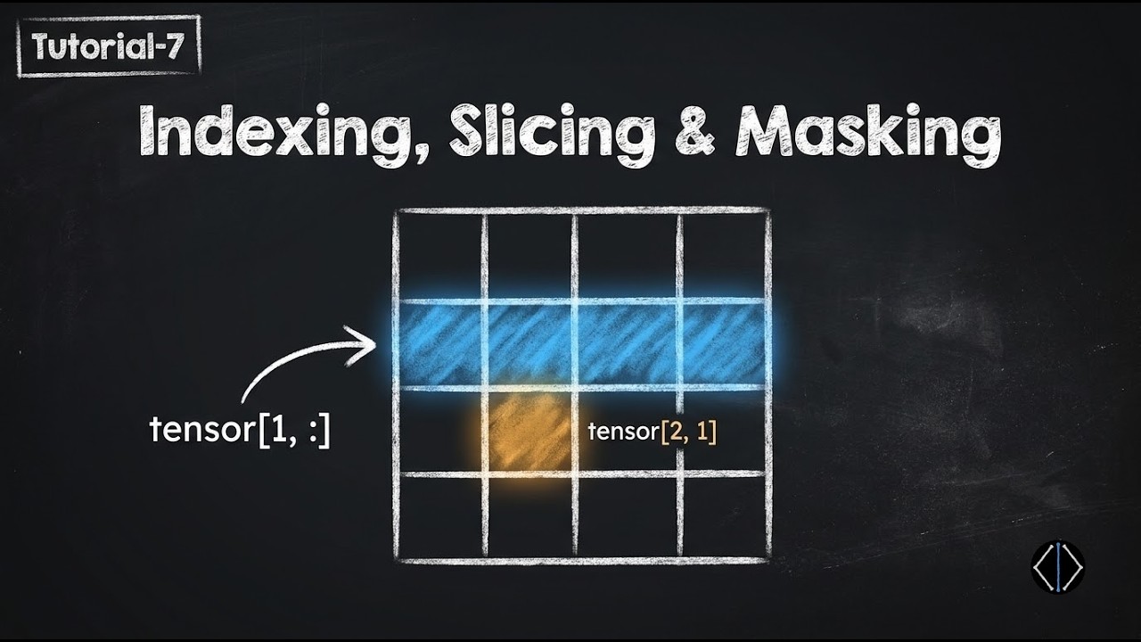
Watch the focused indexing demonstration, then read the examples on ranges. Together, they show how a selection’s values and shape depend on the indices you use.

A slice has the form start:stop:step. The start is included, the stop is excluded, and an omitted step means “take every element.” For example:

patch = x[1:3, :2]
print(patch)
# tensor([[4., 5.],
#         [7., 8.]])
print(patch.shape)  # torch.Size([2, 2])

The first slice chooses rows 1 and 2; the second chooses columns 0 and 1. x[::2, :] would choose every second row.

An integer index removes an axis; a slice retains it. This matters when later code expects a batch axis:

print(x[1].shape)       # torch.Size([3])
print(x[1:2].shape)     # torch.Size([1, 3])
print(x[2, 1].shape)    # torch.Size([]): a zero-dimensional tensor

Use x[1:2] rather than x[1] when you need a batch of one. A single selected value remains a tensor; .item() extracts a Python number if you specifically need one.

You can also select rows using a boolean condition:

row_mask = x[:, 0] > 5
print(row_mask)          # tensor([False, False, True, True])
print(x[row_mask].shape) # torch.Size([2, 3])

Here the mask has one entry per row, so it selects two complete rows. Basic slices can share storage with their source: changing values through a slice can change x. Use .clone() if you need an independent copy, and avoid modifying a source tensor unintentionally.

Change shape while preserving the values

Indexing chooses a subset; reshaping keeps the elements but gives them different dimensions. A valid reshape must preserve the total number of elements.

Watch the reshape examples, concentrating on the element count and the role of a size-one axis. The video also introduces view; for now, use reshape, because view has additional memory-layout restrictions.

Our x has 12 elements. Both of these shapes therefore work:

print(x.reshape(2, 6).shape)  # torch.Size([2, 6])
print(x.reshape(-1).shape)    # torch.Size([12])

In reshape(-1), PyTorch infers the one unspecified size. Reshaping changes how the sequence of values is grouped; it does not exchange the meanings of axes. Do not use it to “swap rows and columns.”

Flattening is especially useful when each example has several axes of features. Suppose a batch contains four examples, each arranged as a 2-by-3 grid:

grids = torch.arange(24, dtype=torch.float32).reshape(4, 2, 3)
flat_features = grids.reshape(4, -1)

print(grids.shape)         # torch.Size([4, 2, 3])
print(flat_features.shape) # torch.Size([4, 6])

The first dimension stays at four, so examples remain separate; the other two dimensions become six features per example. By contrast, grids.reshape(-1) produces one 24-element vector and loses the batch structure.

To add a size-one axis without changing the elements, use unsqueeze:

one_example = x[0]                  # Shape: (3,)
batch_of_one = one_example.unsqueeze(0)
column = one_example.unsqueeze(1)

print(batch_of_one.shape)           # torch.Size([1, 3])
print(column.shape)                 # torch.Size([3, 1])
print(batch_of_one.squeeze(0).shape) # torch.Size([3])

squeeze(0) removes axis 0 only if its size is one. Naming the axis is safer than an unrestricted squeeze() when a batch might contain just one example: an unrestricted call could remove the batch axis too. Finally, do not assume a reshape is an independent copy; depending on the source tensor’s layout, it may share storage.

Reduce along the axis you mean

A reduction combines multiple values, often producing a smaller tensor. The key question is not merely “sum or average?” but which axis should disappear?

Watch the brief demonstration of reductions before applying them to our two-axis tensor.

For x with shape (4, 3), reducing over dim=0 combines the four rows and leaves one value per feature. Reducing over dim=1 combines the three features within each row and leaves one value per example.

feature_totals = x.sum(dim=0)
example_means = x.mean(dim=1)

print(feature_totals)             # tensor([22., 26., 30.])
print(feature_totals.shape)       # torch.Size([3])
print(example_means)              # tensor([ 2.,  5.,  8., 11.])
print(example_means.shape)        # torch.Size([4])

If you omit dim, the operation reduces across all elements:

print(x.mean())        # tensor(6.5000)
print(x.mean().shape)  # torch.Size([])

mean() requires an appropriate floating-point (or complex) tensor; x is floating-point because we created it with decimal values. Other common reductions include sum() and max(). With a specified dimension, x.max(dim=1) supplies both the maximum values and their indices; use .values or .indices to select the result you need.

Sometimes you want to combine values but keep the reduced axis as size one:

row_means = x.mean(dim=1, keepdim=True)
print(row_means.shape)  # torch.Size([4, 1])

That retained axis is useful immediately: it lets one mean line up with each row’s three features.

Broadcast compatible shapes

Elementwise operations such as subtraction ordinarily pair up corresponding entries. Broadcasting extends that idea when one tensor has an absent axis or an axis of size one. It lets us apply a feature-specific value to every example without manually constructing repeated rows.

Start with the visual example, then read the general rule in the PyTorch tutorial.

For each pair of axes, starting on the right, the sizes must match, one size must be 1, or one tensor must lack that axis. The result takes the larger compatible size on each axis.

Here is a direct use of the reductions from the previous section:

feature_means = x.mean(dim=0)  # Shape: (3,)
centered = x - feature_means    # Shapes: (4, 3) and (3,)

print(feature_means)            # tensor([5.5000, 6.5000, 7.5000])
print(centered.shape)           # torch.Size([4, 3])

The final axes both have size three. feature_means lacks a first axis, so its three values are subtracted from each of x’s four rows.

Now consider removing each row’s own mean. x.mean(dim=1) has shape (4,). That does not line up with (4, 3): comparing from the right gives sizes 4 and 3. Retain the reduced axis instead:

row_means = x.mean(dim=1, keepdim=True)  # Shape: (4, 1)
row_centered = x - row_means             # Result shape: (4, 3)

print(row_centered[0])  # tensor([-1.,  0.,  1.])

The size-one second axis allows each row’s mean to be used for all three entries in that row. This is why keepdim=True and unsqueeze() are more than shape conveniences: they can express which values should be paired in a broadcast operation. If an elementwise operation fails with a size mismatch, write both shapes down and compare them from the right before changing the code.

Conclusion

You can now select elements, rows, columns, and ranges; reshape a tensor while preserving its element count; reduce over an intentional axis; and use singleton dimensions to make broadcasting express the calculation you want. The most reliable habit is to check .shape after each operation, especially when an integer index or reduction may remove an axis.

Next, you will use PyTorch autograd to compute gradients. These same tensor operations will then become parts of scalar objectives whose derivatives PyTorch tracks.